Jetson Nano + Sphero RVR Mash-up (PART 2)
 D___Run___
 Example 3: Machine Learning and Collision Avoidance
Our last example that we are going to tackle is putting Jetson Nano to good use and leverage the Machine Learning capabilities!
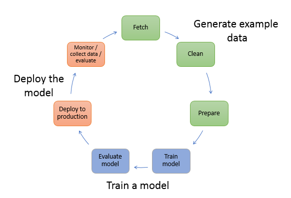
We are going to go through an entire workflow of collecting data using the camera on your bot and if the bot is “blocked” or “Free”. We will then train that model and have your bot use that model to have your RVR avoid objects, edges and other perils in real time. In essence, we are building a safety bubble around our robot with which it will avoid objects that come within that bubble.
This example will take running a couple of different programs, one for each step of the workflow and they are all housed in the Collision Avoidance directory.
Data Collection
Open the directory using the Notebooks files manager. You should see three Notebooks and open the data_collection.ipynb. Once opened, run the Notebook and it should display a live feed of your bot's camera and a simple interface of buttons and text boxes.
We will use this interface to collect camera images of the bot being “blocked” or free. The process works as follows:
- Pick up your robot while the script is running and place it in a situation where it is “blocked”, or about 2-3 inches away from running into an object.
- Click the “Blocked” button. This will capture the image and save it to a directory of images called blocked. The number next to the button should increment by 1.
- Move your bot to a different location and situation where it is blocked and click "Blocked". Again, incrementing the number.
- Repeat this process to collect about 100 or so unique blocked images trying to get as much variation of objects, colors and lighting qualities as possible.
- Repeat the process for the “Free” button as well by placing the robot in a situation where it would be free to drive forward, capture the image, move and repeat for about 100 images.
Code to Note
As with most Python programs we start out by importing the needed packages. This program is no exception! We import a number packages to build our UI inside of Jupyter Notebooks as well as gaining access to our OS.
The packages to really pay attention to here are the the Camera and brg8_to_jpeg packages, which if you did the first example to test your camera, will be familiar.
We also import the uuid package which is used to produce unique and random strings for us to use as file names of our images.
language:python
import os
import traitlets
import ipywidgets.widgets as widgets
from IPython.display import display
from jetbot import Camera, bgr8_to_jpeg
from uuid import uuid1
With the packages imported we can now define and instantiate a few objects. First of all our camera object and we set the image width and height to 224 pixels each as well as setting the frame rate to 10fps. We set it to a lower fps here because we are just capturing still images and don't need a highly responsive video feed. It helps with reducing lag the further you are away from your WiFi router.
Next, we define the image widget which is in JPEG format with the same 224 x 224 size as our camera object.
language:python
camera = Camera.instance(width=224, height=224, fps=10)

image = widgets.Image(format='jpeg', width=224, height=224)  # this width and height doesn't necessarily have to match the camera
With both objects created and defined we then link them together using the Jupyter Notebooks traitlet.dlink() method. This saves us a lot of other programming to pipe the output of the camera and display it in the UI. It also allows us to apply a transform to change the output of the image into something displayable.
language:python
camera_link = traitlets.dlink((camera, 'value'), (image, 'value'), transform=bgr8_to_jpeg)
We will be capturing images of both "Blocked" and "Free" situations. These images will be stored in their own directories within a "dataset" directory. So, we define the path strings here!
language:python
blocked_dir = 'dataset/blocked'
free_dir = 'dataset/free'
We then use the "try/except" statement to catch if we have already created the directories as these next functions can throw an error if the directories exist already
language:python
try:
    os.makedirs(free_dir)
    os.makedirs(blocked_dir)
except FileExistsError:
    print('Directories not created becasue they already exist')
With our dataset directories created we can now define some UI bits and pieces. We define a few buttons to use to trigger the capture of an image as well as define where to save that image (either in the "Free" or "Blocked" directory). We also create and define two text widgets to display how many images are in each of the two directories.
language:python
button_layout = widgets.Layout(width='128px', height='64px')
free_button = widgets.Button(description='add free', button_style='success', layout=button_layout)
blocked_button = widgets.Button(description='add blocked', button_style='danger', layout=button_layout)
free_count = widgets.IntText(layout=button_layout, value=len(os.listdir(free_dir)))
blocked_count = widgets.IntText(layout=button_layout, value=len(os.listdir(blocked_dir)))
Next, we define a few functions for saving the images, building their file names and defining their directory path.
language:python
def save_snapshot(directory):
    image_path = os.path.join(directory, str(uuid1()) + '.jpg')
    with open(image_path, 'wb') as f:
        f.write(image.value)

def save_free():
    global free_dir, free_count
    save_snapshot(free_dir)
    free_count.value = len(os.listdir(free_dir))

def save_blocked():
    global blocked_dir, blocked_count
    save_snapshot(blocked_dir)
    blocked_count.value = len(os.listdir(blocked_dir))
Finally, we attach the functions we just defined as callbacks. We use a 'lambda' function to ignore the parameter that the on_click event would provide to our function because we don't need it.
language:python
free_button.on_click(lambda x: save_free())
blocked_button.on_click(lambda x: save_blocked())
With everything we defined, connected and functional we then display all of the widgets and start the live interface using the display() function!
language:python
display(image)
display(widgets.HBox([free_count, free_button]))
display(widgets.HBox([blocked_count, blocked_button]))
With that you now have a data collection tool for collecting images for computer vision training on your RVR and Jetson Nano. This is a great script to save and keep close by for future projects as it is the basis of defining objects or situations in machine learning.
Think of it this way; this example has two situations: free and blocked. You could expand this code to categorize objects. So, you could define a baseball, a can of soup and your cat. You would then just expand the code to include three options as well as renaming the directories. You can then collect images of those objects for your robot to respond to!
Training the Model
With all of our images (data) collected it is now time to create and train the model on our Jetson Nano. This is one of the things that makes the NVIDIA Jetson Nano special; it is both what you use to run a model, but also the GPU that you use to train it. You don't need to do all of your training in the cloud or on an expensive desktop machine.
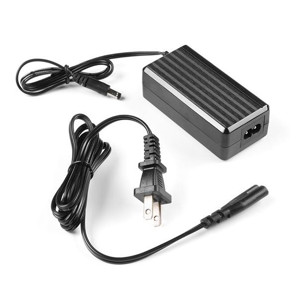
One thing we do recommend here is that you switch how you power your Nano to an outlet power based 5V/4A power supply during the training process. We have done training on the battery, but it is not ideal and technically out of spec for the process.
With the power supply swapped out, open up the model_trainiing.ipynb Notebook from the file manager in Jupyter Notebooks. This program will do very little in terms of outputting any information for you, so be patient. When you run this script you will see a few outputs that state that the Nano is downloading a few things, which is fine.
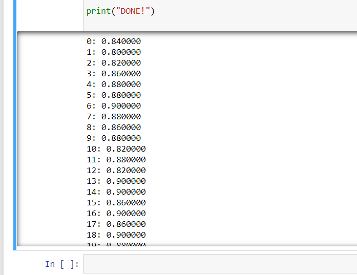
Once all of the errors are cleared the script will start training epochs, 30 of them. When each epoch is complete you will see a report printed out giving an accuracy level of the epoch test. Once the training is complete you will see it print “DONE!” and you will also see that a final model file is created in the project directory named “XXXX”.
Code to Note
This Python script is a little boring when it comes to output in Jupyter Notebooks, but it is probably the most important and pivotal part in this whole project. This script creates the machine learning model that our robot will use to define if it is "Blocked" or "Free".
We start out by importing a number of Python packages which includes a number of packages for torch and torchvision. These are packages for doing machine learning and building models like the one we are doing here. Essentially, each step we take in the process of building our model requires its own package.
language:python
import torch
import torch.optim as optim
import torch.nn.functional as F
import torchvision
import torchvision.datasets as datasets
import torchvision.models as models
import torchvision.transforms as transforms
First up is defining our dataset that we will be training our model against. We define the dataset by pointing it to a specific ImageFolder that we have created called dataset. We then apply a number of transforms to our images to get everything to correct size and format.
language:python
dataset = datasets.ImageFolder(
    'dataset',
    transforms.Compose([
        transforms.ColorJitter(0.1, 0.1, 0.1, 0.1),
        transforms.Resize((224, 224)),
        transforms.ToTensor(),
        transforms.Normalize([0.485, 0.456, 0.406], [0.229, 0.224, 0.225])
    ])
)
Once our dataset is defined and in the correct format it is now time to split that dataset in two. The first dataset in our training set and the second set are the sets we will be testing our model against. We define both of those here as well as the parameters for each DataLoader.
language:python
train_dataset, test_dataset = torch.utils.data.random_split(dataset, [len(dataset) - 50, 50])

train_loader = torch.utils.data.DataLoader(
    train_dataset,
    batch_size=16,
    shuffle=True,
    num_workers=4
)

test_loader = torch.utils.data.DataLoader(
    test_dataset,
    batch_size=16,
    shuffle=True,
    num_workers=4
)
Once our datasets have been defined and loaded we can further define our model we are looking to use. For this we will be using the alexnet model that is pre-trained and that we are looking for our two defined situations we have defined as "Free" and "Blocked". If we had more than these two we would need to change the last number in torch.nn.Linear(model.classifier[6].in_features, 2) to whatever the number of outcomes we were looking for!
language:python
model = models.alexnet(pretrained=True)
model.classifier[6] = torch.nn.Linear(model.classifier[6].in_features, 2)
We then define the number of epochs or how many times to train our model. For this first go we are running 30 epochs, you can adjust this up or down as you refine your model. We are also defining the file name for our model that we are creating as a file called best_model.pth.
language:python
NUM_EPOCHS = 30
BEST_MODEL_PATH = 'best_model.pth'
best_accuracy = 0.0
Now, for each epoch we run the training against all of our images in our training loader and then test the model against the data in our test loader. For each epoch you will see the printout of the epoch number and the accuracy level of the model. This will change as the number of epochs are ran with only the highest accuracy model being saved as our best_model.pth file.
language:python
for epoch in range(NUM_EPOCHS):

    for images, labels in iter(train_loader):
        images = images.to(device)
        labels = labels.to(device)
        optimizer.zero_grad()
        outputs = model(images)
        loss = F.cross_entropy(outputs, labels)
        loss.backward()
        optimizer.step()

    test_error_count = 0.0
    for images, labels in iter(test_loader):
        images = images.to(device)
        labels = labels.to(device)
        outputs = model(images)
        test_error_count += float(torch.sum(torch.abs(labels - outputs.argmax(1))))

    test_accuracy = 1.0 - float(test_error_count) / float(len(test_dataset))
    print('%d: %f' % (epoch, test_accuracy))
    if test_accuracy > best_accuracy:
        torch.save(model.state_dict(), BEST_MODEL_PATH)
        best_accuracy = test_accuracy

print("DONE!")
Like the data collection script, this script is universally useful when it comes to situational and object detection for your robot! Keep this script handy to modify as you modify your data collection script. The only thing you would really need to change in this script would be changing the final number in this line of code...
model.classifier[6] = torch.nn.Linear(model.classifier[6].in_features, 2)
Instead of 2, you would change it to how many different categories you are collecting. So for our three examples of baseball, cat and can of soup, that number would be 3.
Deploying the Model
With our data collected and our machine learning model created it is now time to put it all together and see if our bot can drive around and use the model to avoid objects. From the Object Avoidance project directory open the live_demo.ipynb file and run it.
After a bit the code should execute and your robot should start driving about. In the Notebook you should see the live feed from the camera as it drives around. In your code the Jetson Nano is taking each frame of the camera and evaluating whether the bot is “Blocked” or "Free". If you place something in front of your bot it should turn to the left and avoid that object. This should work for instances that you took photos of “Blocked” and “Free”, so if you never took a picture of a ledge or edge of a table as “Blocked” the robot will not think it is blocked and run off of the edge!
We recommend starting your bot out in a safe place where there are few obstacles. If the model is not performing to your expectations, that is OK, ours didn’t either! Stop the live demo and collect more images of “Blocked” and “Free” scenarios and then retrain the model using the same process that you have gone through.
Code to Note
Now, we are going to bring everything together in terms of our Python script. While that is awesome and the end all, be all goal of this whole project, it does get messy and complicated. Let's dive in and take a look at what this looks like.
First off, like always we are importing the required packages to make everything work. This includes packages for using the OS, all of our Jupyter Notebook widgets, machine learning and computer vision functionality as well the RVR SDK. Fewww... it's a lot of modules!
language:python
import os
import sys

import torch
import torchvision
import cv2
import numpy as np
import traitlets
from IPython.display import display
import ipywidgets.widgets as widgets
from jetbot import Camera, bgr8_to_jpeg
import torch.nn.functional as F
import time

from sphero_sdk import SpheroRvrObserver
from sphero_sdk import Colors
from sphero_sdk import RvrLedGroups
Before we forget about the simple stuff, we instantiate the RVR as an observer and then send the command to wake it up!
language:python
rvr = SpheroRvrObserver()
rvr.wake()
Next we are going to get our machine learning model setup and ready to use. Like in our training we define the model to use as Alexnet, but this time it is not pre-trained. We state that we are looking for two defined features ("Free" and "Blocked") and that we will be using our training model that we created "best_model.pth".
language:python
model = torchvision.models.alexnet(pretrained=False)
model.classifier[6] = torch.nn.Linear(model.classifier[6].in_features, 2)

model.load_state_dict(torch.load('best_model.pth'))
We then define a function for transforming an image that we will be capturing from the camera frame and getting it into the proper format to be run through our machine learning model.
language:python
def preprocess(camera_value):
    global device, normalize
    x = camera_value
    x = cv2.cvtColor(x, cv2.COLOR_BGR2RGB)
    x = x.transpose((2, 0, 1))
    x = torch.from_numpy(x).float()
    x = normalize(x)
    x = x.to(device)
    x = x[None, ...]
    return x
We then create and define a number of our Jupyter Notebook widgets for us to interface with. This includes our JetBot camera here as well as the image widget and a slider to display the probability of an image being "Blocked" or "Free" in real time. Like before, we then link the camera and image together so we can simply display the camera view and then we display everything at once using the display() function.
language:python
camera = Camera.instance(width=224, height=224)
image = widgets.Image(format='jpeg', width=224, height=224)
blocked_slider = widgets.FloatSlider(description='blocked', min=0.0, max=1.0, orientation='vertical')

camera_link = traitlets.dlink((camera, 'value'), (image, 'value'), transform=bgr8_to_jpeg)

display(widgets.HBox([image, blocked_slider,bat_slider]))
We define the update() function that we will be using as a callback function. This function is what ties all of this together in terms of the application and logic behind the robot avoiding being "Blocked". First off, on change the function takes the new image data that it is passed and processes it through the preprocess function we created before. Once processed, we plug that into our model. The output of the model function is then run through a softmax function to normalize it to build a probability distributions (a sum total of 1).
We then define the probability of the image as "Blocked" as the first value in the model. The value of the probability slider is then set to that value.
Using that value we use a basic if statement to evaluate it against a probability of 50%. If the probability is less than 50% then the robot drives straight forward with its lights set to green. If it is higher than 50% the robot LEDs turn red and it pivots to the left.
language:python
def update(change):
    global blocked_slider
    x = change['new']
    x = preprocess(x)
    y = model(x)

    y = F.softmax(y, dim=1)

    prob_blocked = float(y.flatten()[0])
    blocked_slider.value = prob_blocked

    if prob_blocked < 0.5:
        rvr.raw_motors(1,64,1,64)
        rvr.led_control.set_all_leds_color(color=Colors.green)
        #forward
    else:
        rvr.raw_motors(2,128,1,128)
        rvr.led_control.set_all_leds_color(color=Colors.red)
        #left
    time.sleep(0.001)
To start the function look we call the update() function now, before basing it off of the observe() callback method of the camera.
language:python
update({'new': camera.value})  # we call the function once to intialize
We finally attach the update() function to the camera.observe() method to be called each time there is a new image value (which is roughly 30 times per second)!
language:python
camera.observe(update, names='value')  # this attaches the 'update' function to the 'value' traitlet of our camera
Fewwww... we now have a fully functional robot that is using Machine Learning to navigate the world around it! Now it is time for you to explore the Sphero SDK a little more indepth and make this program your own! We drive around and change color, but there are a number of other functional parts to the robot you can use as well as a whole suite of sensors on the RVR we haven't even put to use yet. Be sure to explore more and build on this foundational project!