Graph Sensor Data with Python and Matplotlib

Contributors: Shawn Hymel

Plot Sensor Data

In the Python Programming Tutorial: Getting Started with the Raspberry Pi, the final example shows how to sample temperature data from the TMP102 once per second over 10 seconds and then save that information to a comma separated value (csv) file. To start plotting sensor data, let's modify that example to collect data over 10 seconds and then plot it (instead of saving it to a file).

TMP102 Module

In order to simplify I²C reading and writing to the TMP102, we will create our own TMP102 Python module that we can load into each of our programs. Open a new file named tmp102.py:

language:shell
nano tmp102.py

Copy in the following Python code:

language:python
import smbus

# Module variables
i2c_ch = 1
bus = None

# TMP102 address on the I2C bus
i2c_address = 0x48

# Register addresses
reg_temp = 0x00
reg_config = 0x01

# Calculate the 2's complement of a number
def twos_comp(val, bits):
    if (val & (1 << (bits - 1))) != 0:
        val = val - (1 << bits)
    return val

# Read temperature registers and calculate Celsius
def read_temp():

    global bus

    # Read temperature registers
    val = bus.read_i2c_block_data(i2c_address, reg_temp, 2)
    temp_c = (val[0] << 4) | (val[1] >> 4)

    # Convert to 2s complement (temperatures can be negative)
    temp_c = twos_comp(temp_c, 12)

    # Convert registers value to temperature (C)
    temp_c = temp_c * 0.0625

    return temp_c

# Initialize communications with the TMP102
def init():

    global bus

    # Initialize I2C (SMBus)
    bus = smbus.SMBus(i2c_ch)

    # Read the CONFIG register (2 bytes)
    val = bus.read_i2c_block_data(i2c_address, reg_config, 2)

    # Set to 4 Hz sampling (CR1, CR0 = 0b10)
    val[1] = val[1] & 0b00111111
    val[1] = val[1] | (0b10 << 6)

    # Write 4 Hz sampling back to CONFIG
    bus.write_i2c_block_data(i2c_address, reg_config, val)

    # Read CONFIG to verify that we changed it
    val = bus.read_i2c_block_data(i2c_address, reg_config, 2)

Save the code with ctrl + x, press y, and press enter. This allows us to call the init() and read_temp() functions to easily get temperature (in Celsius) from the TMP102.

Temperature Logging and Graphing

In the same directory as the tmp102.py file, create a new file (using your favorite editor), and paste in the following code:

language:python
import time
import datetime as dt
import matplotlib.pyplot as plt
import tmp102

# Create figure for plotting
fig = plt.figure()
ax = fig.add_subplot(1, 1, 1)
xs = []
ys = []

# Initialize communication with TMP102
tmp102.init()

# Sample temperature every second for 10 seconds
for t in range(0, 10):

    # Read temperature (Celsius) from TMP102
    temp_c = round(tmp102.read_temp(), 2)

    # Add x and y to lists
    xs.append(dt.datetime.now().strftime('%H:%M:%S.%f'))
    ys.append(temp_c)

    # Wait 1 second before sampling temperature again
    time.sleep(1)

# Draw plot
ax.plot(xs, ys)

# Format plot
plt.xticks(rotation=45, ha='right')
plt.subplots_adjust(bottom=0.30)
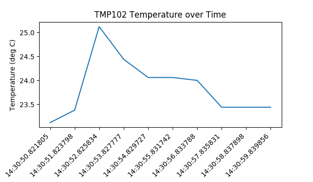
plt.title('TMP102 Temperature over Time')
plt.ylabel('Temperature (deg C)')

# Draw the graph
plt.show()

Save (give it a name like tempgraph.py) and exit. Run the program with:

language:shell
python tempgraph.py

Wait while the program collects data (about 10 seconds). Feel free to breathe on or fan near the temperature sensor to change the ambient temperature (gives you some interesting data to look at). Once the collection has finished, you should be presented with a plot showing how the temperature changed over time.

Code to Note

We create the graph in a very similar manner to the Formatting example in Introduction to Matplotlib. The only difference is that we build the xs and ys lists programmatically. Each second, the temperature is read from the TMP102 sensor and appended to the ys list. The local time (of the Raspberry Pi) is captured with dt.datetime.now() and appended to the xs list.

The xs and ys lists are then used to create a plot with ax.plot(xs, ys). Note that we are explicitly creating a figure and a single set of axes (instead of calling the plt.plot() shortcut). We will use the handle to the axes in the next sections when we look at animating the plot.