Sound Location Part 2 with the Qwiic Sound Trigger and the u-blox ZED-F9x

Contributors: PaulZC

Here There Be Dragons!

Sound_Trigger_Analyzer_2D.py can work with any configuration of the trigger positions (so long as the X coordinate of C is between A and B). They do not need to be arranged in a nice right-angled triangle with A-C pointing North. Don’t believe me? Want proof? Good for you! OK. Brace yourself. Here we go… Here is the actual math used in Sound_Trigger_Analyzer_2D.py.

Sensor Coordinates

Let’s suppose our three sound triggers are arranged such that they form a triangle ABC:

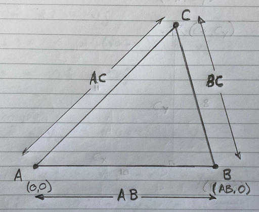
We know the length of the sides: AB, AC and BC.

We know the coordinates of A and B. A is our origin and is located at (0,0). B is due ‘East’ of A and defines our X axis. So we say that B is located at (AB,0). But we don’t yet know the location of C. We need to calculate it. Let’s call the location of C (C_X,C_Y).

If we draw a line from C so it meets line A-B at right angles:

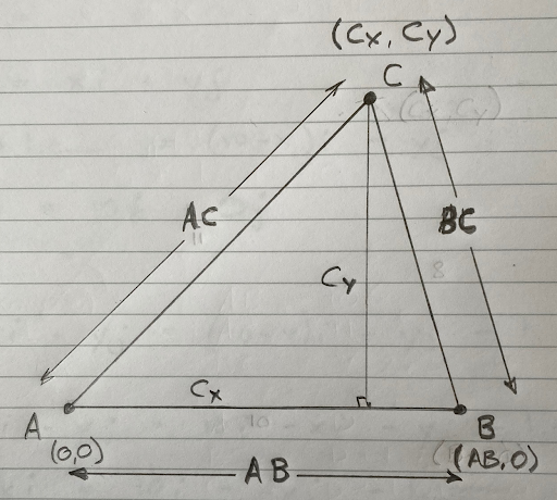
Pythagoras’ Theorem tells us that:

• Equation 1: AC² = C_X² + C_Y²
• Equation 2: BC² = ( AB - C_X )² + C_Y²

If we rearrange those equations, bringing C_Y² to the left and multiplying out the brackets, we get:

• C_Y² = AC² - C_X²
• C_Y² = BC² - AB² + 2.AB.C_X - C_X²

Because those two equations are equal, we can arrange them as:

• AC² - C_X² = BC² - AB² + 2.AB.C_X - C_X²

The two -C_X² cancel out. Rearranging, we get:

• C_X = ( AC² - BC² + AB² ) / 2.AB

We can find C_Y by inserting the value for C_X into one of our earlier equations:

• C_Y² = AC² - C_X²

So:

• C_Y = √ ( AC² - C_X² )

We now have the coordinates for C: ( C_X , C_Y )

Sound Event Timings

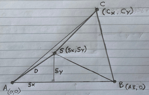
Now, let’s suppose our sound trigger system is running and it detects a sound. Let’s call the location of the sound S and give it coordinates ( S_X , S_Y ):

Our three systems are logging the time the sound arrives at each sensor (very accurately!).

The time taken for the sound to reach A is: the distance from S to A divided by the speed of sound. Likewise for B and C.

If all three systems hear the sound at the exact same time, then we know that the sound took an equal time to travel from S to A, B and C. That’s a special case where the distances SA, SB and SC are equal (equidistant). But usually sensors B and C will hear the sound at different times to A due to the distances SB and SC being different to SA. We need to include those differences in distance in our calculation. To save some typing, let’s call the distance SA: D

• SB = D + D_diffB
• SC = D + D_diffC

D_diffB is the difference between SB and D. Likewise, D_diffC is the difference between SC and D. Note that D_diffB or D_diffC could be negative if the source of the sound is closer to B or C than A.

Sensors B and C will hear the sound earlier or later than A depending on D_diffB and D_diffC.

What we do not know is how long the sound took to travel from S to A, because we do not know the distance D. That’s what we need to calculate,

What we do know is the difference in the time of arrival of the sound at our three sensors. If we bring the three sets of sensor data together, we can calculate the difference in the time of arrival at each sensor. Let’s say that:

• The time recorded by trigger A is timeA
• The time recorded by trigger B is timeB
• The time recorded by trigger C is timeC

Let’s calculate the differences in those times:

• T_diffB = timeB - timeA
• T_diffC = timeC - timeA

Again, T_diffB and T_diffC could be negative if the source of the sound is closer to B or C than A.

Sound Event Coordinates

We can convert those differences in time into differences in distance by multiplying by the speed of sound:

• D_diffB = T_diffB * speed_of_sound
• D_diffC = T_diffC * speed_of_sound

Now we can use Pythogoras’ Theorem as before to study our triangles:

• D² = S_X² + S_Y²
• (D + D_diffB)² = (AB - S_X)² + S_Y²

We need to add an extra triangle to include SC:

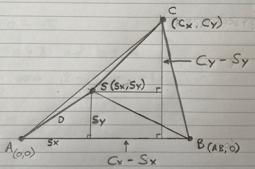
The width of the new triangle is:

• C_X - S_X

The height of the new triangle is:

• C_Y - S_Y

So, using Pythagoras’ Theorem again:

• (D + D_diffC)² = (C_X - S_X)² + (C_Y - S_Y)²

We now have our three equations:

• Equation 3: D² = S_X² + S_Y²
• Equation 4: (D + D_diffB)² = (AB - S_X)² + S_Y²
• Equation 5: (D + D_diffC)² = (C_X - S_X)² + (C_Y - S_Y)²

We need to solve for D. To begin, let’s substitute the value for S_Y² from the second equation into the first equation, so we can find the relationship between D and S_X:

• D² = S_X² + (D + D_diffB)² - (AB - S_X)²

Multiplying out the brackets, that becomes:

• D² = S_X² + D² + 2.D_diffB.D + D_diffB² - AB² + 2.AB.S_X - S_X²

As before, the D² cancel and so do the S_X² leaving:

• 0 = 2.D_diffB.D + D_diffB² - AB² + 2.AB.S_X

Rearranging:

• 2.AB.S_X = AB² - 2.D_diffB.D - D_diffB²

Divide through by 2.AB:

• S_X = ( AB² - 2.D_diffB.D - D_diffB² ) / 2.AB

Let’s make life easier for ourselves and say that:

• Equation 6: S_X = S_Xa.D + S_Xb

Where:

• S_Xa = ( -2.D_diffB ) / 2.AB
• S_Xb = ( AB² - D_diffB² ) / 2.AB

We can calculate both values because we know AB and can calculate D_diffB:

• D_diffB = T_diffB * speed_of_sound = ( timeB - timeA ) * speed_of_sound

Looking at equation 3 again:

• D² = S_X² + S_Y²

If we replace S_X with ( S_Xa.D + S_Xb ), we get:

• D² = ( S_Xa.D + S_Xb )² + S_Y²

Rearranging:

• S_Y² = D² - ( S_Xa.D + S_Xb )²

Multiplying out the bracket, it becomes:

• S_Y² = D² - S_Xa².D² - 2.S_Xa.S_Xb.D - S_Xb²

Simplifying:

• S_Y² = ( 1 - S_Xa² ).D² - 2.S_Xa.S_Xb.D - S_Xb²

So:

• Equation 7: S_Y = √ ( ( 1 - S_Xa² ).D² - 2.S_Xa.S_Xb.D - S_Xb² )

That’s ever so slightly horrible, but let’s go with it…

Now we have values for S_X and S_Y in terms of D, which we can plug into equation 5:

• (D + D_diffC)² = (C_X - S_X)² + (C_Y - S_Y)²

Substituting for S_X and S_Y we get:

• (D + D_diffC)² = (C_X - ( S_Xa.D + S_Xb ) )² + (C_Y - √ ( ( 1 - S_Xa² ).D² - 2.S_Xa.S_Xb.D - S_Xb² ) )²

Multiplying out the brackets gives (brace yourself!):

• D² + 2.D_diffC.D + D_diffC² = C_X² - 2.C_X.S_Xa.D - 2.C_X.S_Xb + S_Xa².D² + 2.S_Xa.S_Xb.D + S_Xb² + C_Y² - 2.C_Y.√ ( ( 1 - S_Xa² ).D² - 2.S_Xa.S_Xb.D - S_Xb² ) + ( 1 - S_Xa² ).D² - 2.S_Xa.S_Xb.D - S_Xb²

Simplifying and moving everything but the root to the left gives:

• ( 1 - S_Xa² - ( 1 - S_Xa² )).D² + ( 2.D_diffC + 2.C_X.S_Xa - 2.S_Xa.S_Xb + 2.S_Xa.S_Xb).D + D_diffC² - C_X² + 2.C_X.S_Xb - S_Xb² - C_Y² + S_Xb² = -2.C_Y.√ ( ( 1 - S_Xa² ).D² - 2.S_Xa.S_Xb.D - S_Xb² )

Fortunately the D² term cancels out completely, which is good news. If it didn’t, we’d have a quartic equation to solve instead of a quadratic…

Simplifying:

• ( 2.D_diffC + 2.C_X.S_Xa).D + D_diffC² - C_X² + 2.C_X.S_Xb - C_Y² = -2.C_Y.√ ( ( 1 - S_Xa² ).D² - 2.S_Xa.S_Xb.D - S_Xb² )

Dividing through by -2.C_Y gives:

• ( ( 2.D_diffC + 2.C_X.S_Xa ).D + D_diffC² - C_X² + 2.C_X.S_Xb - C_Y² ) / -2.C_Y = √ ( ( 1 - S_Xa² ).D² - 2.S_Xa.S_Xb.D - S_Xb² )

We now need to square both sides to get rid of the root. Painful… But we need to do it… But first, to make life easier for ourselves, let’s simplify further and say:

• da.D + db = √ ( ( 1 - S_Xa² ).D² - 2.S_Xa.S_Xb.D - S_Xb² )

Where:

• da = ( 2.D_diffC + 2.C_X.S_Xa ) / -2.C_Y
• db = ( D_diffC² - C_X² + 2.C_X.S_Xb - C_Y² ) / -2.C_Y

Remember that we can already calculate values for da and db because we know or can calculate values for: D_diffC; C_X; S_Xb; and C_Y.

Square both sides:

• da².D² + 2.da.db.D + db² = ( 1 - S_Xa² ).D² - 2.S_Xa.S_Xb.D - S_Xb²

Moving the terms on the right over to the left:

• ( da² - ( 1 - S_Xa² ) ).D² + ( 2.da.db + 2.S_Xa.S_Xb ).D + db² + S_Xb² = 0

That’s a quadratic equation which we can solve in the usual way. Let’s make:

• qa = da² - 1 + S_Xa²
• qb = 2.da.db + 2.S_Xa.S_Xb
• qc = db² + S_Xb²

Remember that we can already calculate values for qa, qb and qc because we already know: da; S_Xa; db; and S_Xb.

Solving the quadratic::

• D = ( -qb +/- √( qb² - 4.qa.qc ) ) / 2.qa

That gives us two possible values for D. One will be negative or otherwise invalid, leaving us with a value for D.

We can then plug the value for D into equation 6 to find the X coordinate of S because we already know the values of S_Xa and S_Xb:

• S_X = S_Xa.D + S_Xb

We can then calculate the Y coordinate of S using equation 3:

• D² = S_X² + S_Y²
• S_Y = √( D² - S_X² )

Enjoy your coordinates!