Lessons in Algorithms

Introduction

Earlier this year, Nathan Seidle, founder of SparkFun, created the Crowdsourcing Algorithms Challenge (aka, the Speed Bag Challenge). After numerous fantastic entries, one was chosen. The winner, Barry Hannigan, was asked to write up his process involved in solving this problem. This article is Barry Hannigan's winning approach to solving real-world problems, even when the problem is not tangibly in front of you.

Firmware Resources

You can view Barry's code by clicking the link below.

As the winner of Nate’s Speed Bag Challenge, I had the wonderful opportunity to meet with Nate at SparkFun's headquarters in Boulder, CO. During our discussions, we thought it would be a good idea to create a tutorial describing how to go about solving a complex problem in an extremely short amount of time. While I’ll discuss specifics to this project, my hope is that you’ll be able to apply the thought process to your future projects---big or small.

Where to Start

In full-fledged software projects, from an Engineer's perspective, you have four major phases:

• Requirements
• Design
• Implementation
• Test

Let’s face it; the design and coding is what everyone sees as interesting, where their creative juices can flow and the majority of the fun can be had. Naturally, there is the tendency to fixate on a certain aspect of the problem being solved and jump right in designing and coding. However, I will argue that the first and last phase can be the most important in any successful project, be it large or small. If you doubt that, consider this: my solution to the speed bag problem was designed wickedly fast, and I didn’t have a bag to test it on. But, with the right fixes applied in the end, the functionality was tested to verify that it produced the correct results. Conversely, a beautiful design and elegant implementation that doesn’t produce the required functionality will surely be considered a failure.

I didn’t mention prototype as a phase, because depending on the project it can happen in different phases or multiple phases. For instance, if the problem isn’t fully understood, a prototype can help figure out the requirements, or it can provide a proof of concept, or it can verify the use of a new technology. While important, prototyping is really an activity in one or more phases.

Getting back to the Speed Bag Challenge, in this particular case, even though it is a very small project, I suggest that you spend a little time in each of the four areas, or you will have a high probability of missing something important. To get a full understanding of what’s required, let's survey everything we had available as inputs. The web post for the challenge listed five explicit requirements, which you can find here. Next, there was a link to Nate’s Github repository that had information on the recorded data format and a very brief explanation of how the speed bag device would work.

In this case, I would categorize what Nate did with the first speed bag counter implementation as a prototype to help reveal additional requirements. From Nate’s write-up on how he built the system, we know it used an accelerometer attached to the base of a speed bag and that the vibration data samples about every 2ms are to be used to count punches. We also now know that applying a polynomial smoothing function and looking for peaks above a threshold doesn't accurately detect punches.

While trying not to be too formal for a small project, I kept these objectives (requirements) in mind while working the problem:

• The algorithm shall be able to produce the correct number of hits from the recorded data sets
• The solution shall be able to run on 8-bit and 32-bit micros
• Produce documentation and help others learn from the solution put forth
• Put code and documents in a public repository or website
• Disclose the punch count and the solution produced for the Mystery data sets
• Accelerometer attached to top of speed bag base, orientation unknown except +Z is up -Z is down
• Complex data patterns will need more than polynomial filtering; you need to adjust to incoming data amplitude variations---as Nate suspects, resonance is the likely culprit
• You have 15 days to complete (Yikes!)

Creating the Solution

As it goes in all projects, now that you know what should be done, the realization that there isn’t enough time sets in. Since I didn't have the real hardware and needed to be able to visually see the output of my algorithm, I started working it out quickly in Java on my PC. I built in a way to plot the results of the waveforms on my screen. I’ve been using NetBeans for years to do Java development, so I started a new speed bag project. I always use JFreeChart library to plot data, so I added it to my project. Netbeans has a really good IDE and built-in GUI designer. All I had to do was create a GUI layout with a blank panel where I want the JFreeChart to display and then, at run time, create the JFreeChart object and add it to the panel. All the oscilloscope diagrams in this article were created by the JFreeChart display. Here is an image from my quick and dirty oscilloscope GUI design page.

This algorithm was needed in a hurry, so my first pass is to be very object oriented and use every shortcut afforded me by using Java. Then, I’ll make it more C like in nature as I nail down the algorithm sequence. I jumped right in and plotted the X, Y and Z wave forms as they came from the recorded results. Once I got a look at the raw data, I decided to remove any biases first (i.e., gravity) and then sum the square of each waveform and take the square root. I added some smoothing by way of averaging a small number of values and employed a minimum time between threshold crossings to help filter out spikes. All in all, this seemed to make the data even worse on the plot. I decided to throw away X and Y, since I didn’t know in what orientation it was mounted and if it would be mounted the same on different speed bag platforms anyway. To my horror, even with just the Z axis, it still just looked like a mess of noise! I’m seeing peaks in the data way too close together. Only my minimum time between thresholds gate is helping make some sense of the punch count, but there really isn’t anything concrete in the data. Something's not adding up. What am I missing?

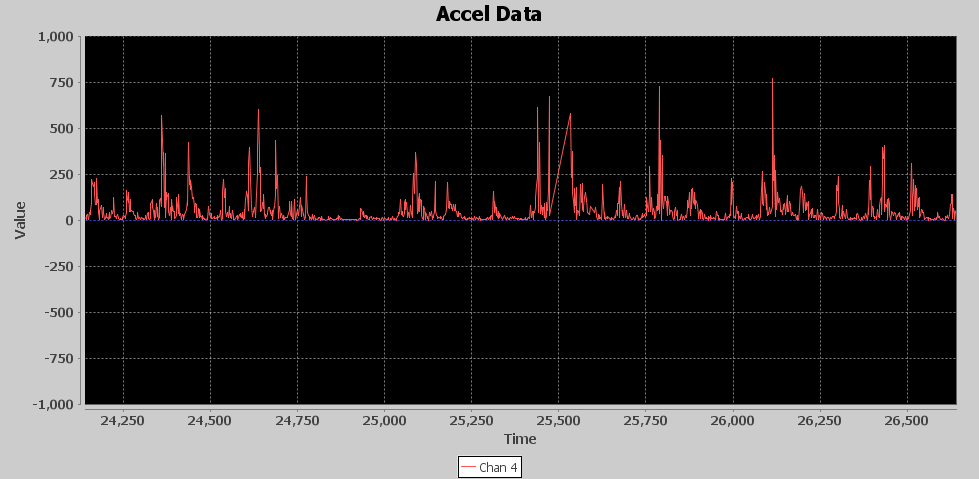
Below is an image of the runF1 waveform. The blue signal is the filtered z axis, and the red line is a threshold for counting punches. As I mentioned, if it weren’t for my 250ms minimum between punch detections, my counter would be going crazy. Notice the way I have introduced two 5 millisecond delays in my runF1() processing so thresholding would be a little better if the red line were moved to the right by 10 milliseconds. I’ll talk more about aligning signals later in this article, but you can see in this image how time aligning signals is crucial for getting accurate results.

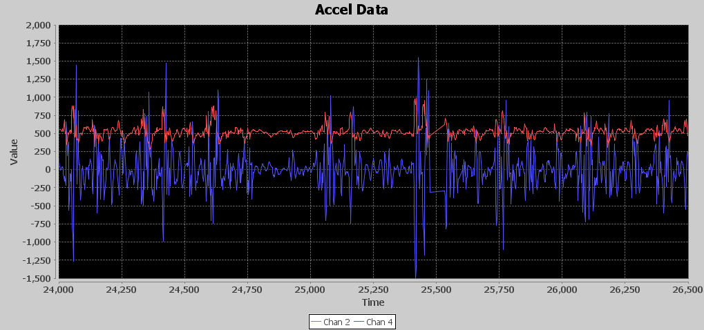
If you look at the virtual oscilloscope output, you can see that between millisecond 25,000 and 26,000, which is 1 second in time, there are around nine distinct acceleration events. No way Nate is throwing nine punches in a second. Exactly how many punches should I expect to see per second? Back to the drawing board. I need another approach. Remember humility is your friend; if you just rush in on your high horse you usually will be knocked off it in a hurry.

Understand the Domain

Typically the requirements are drafted in the context of the domain of the problem that's being solved, or some design aspects are developed from a requirement with domain knowledge applied. I don’t know the first thing about boxing speed bags, so time to do some Googling.

The real nugget I unearthed was that a boxer hits a speed bag, and it makes three contacts with the base: once forward (in punch direction), then it comes all the way back (opposite of punch direction) and strikes the base, and then it goes all the way forward again striking the base (in punch direction). Then the boxer punches it on its way back toward the boxer. This actually gives four opportunities to generate movement to the base, once from the shock of the boxer contacting the bag, and then three impacts with the base.

Now, what I see on the waveforms makes more sense. There isn’t a shock of the bag hitting the base once per punch. My second thought was how many punches can a boxer throw at a speed bag per second. Try as I might, I could not find a straight answer to this question. I found lots of websites with maximum shadow boxing punches and actual punches being thrown maximums but not a maximum for a speed bag. Time to derive my own conclusion: I thought about how far the speed bag must travel per punch and concluded that there must be a minimum amount of force to make the bag travel the distance it needs to impact the base three times. Since I’m not a boxer, all I could do is visualize hitting the bag as slowly as possible and it making three contacts. I concluded from the video in my mind’s eye that it would be difficult to hit a bag less than twice per second. OK, that’s a minimum; how about a maximum? Again, I summoned my mind’s eye video and this time moved my fist to strike the imaginary bag. I concluded with the distance the bag needed to travel and the amount of time to move a fist in and out of the path of the bag that about four per second is all that is possible, even with a skilled boxer. OK, it’s settled. I need to find events in the data that are happening between 2 and 4 hertz. Time to get back to coding and developing!

Build a little, Test a little, Learn a lot

While everyone’s brain works a little differently, I suggest that you try an iterative strategy, especially when you are solving a problem that does not have a clearly defined methodology going into it. I also suggest that when you feel you are ready to make a major tweak to an algorithm, you make a copy of the algorithm before starting to modify the copy, or start with an empty function and start pulling in pieces of the previous iteration. You can use source control to preserve your previous iteration, but I like having the previous iteration(s) in the code so I can easily reference it when working on the next iteration. I usually don’t like to write more than 10 or 20 lines of code without at minimum verifying it complies, but I really want to run it and print something out as confirmation that my logic and assumptions are correct. I’ve done this my entire career and will usually complain if I don’t have target hardware available to actually run what I’m coding. Around 2006, I heard a saying from a former Rear Admiral:

I really identify with that statement, as it succinctly states why I always want to keep running and testing what I’m writing. It either allows you to confirm your assumptions or reveals you are heading down the wrong path, allowing you to quickly get on the right path without throwing away a lot of work. This was yet another reason that I chose Java as my prototype platform, as I could quickly start running and testing code plus graph it out visually, in spite of not having the actual speed bag hardware.

Additionally, you will see in the middle of all six runFx() functions there is code that keeps track of the current time in milliseconds and verifies that the time stamp delta in milliseconds has elapsed or it sleeps for 1 millisecond. This allowed me to watch the data scroll by in my Java plotting window and see how the filtering output looks. I passed in X, Y and Z acceleration data along with an X, Y and Z average value. Since I only used Z data in most algorithms, I started cheating and sending in other values to be plotted, so it’s a little confusing when looking at the graphs of one through five since they don’t match the legend. However, plotting in real time allowed me to see the data and watch the hit counter increment. I could actually see and feel a sense of the rhythm into which the punches were settling and how the acceleration data was being affected by the resonance at prolonged constant rhythm. In addition to the visual output using the Java System.out.println() function, I can output data to a window in the NetBeans IDE.

If you look in the Java subdirectory in my GitHub repository, there is a file named MainLoop.java. In that file, I have a few functions named run1() through run6(). These were my six major iterations of the speed bag algorithm code.

Here are some highlights for each of the six iterations.

runF1

runF1() used only the Z axis, and employed weak bias removal using a sliding window and fixed amplification of the filtered Z data. I created an element called delay, which is a way to delay input data so it could be aligned later with output of averaged results. This allowed the sliding window average to be subtracted from Z axis data based on surrounding values, not by previous values. Punch detection used straight comparison of amplified filter data being greater than average of five samples with a minimum of 250 milliseconds between detections.

runF2

runF2() used only Z axis, and employed weak bias removal via a sliding window but added dynamic beta amplification of the filtered Z data based on the average amplitude above the bias that was removed when the last punch was detected. Also, a dynamic minimum time between punches of 225ms to 270ms was calculated based on delta time since last punch was detected. I called the amount of bias removed noise floor. I added a button to stop and resume the simulation so I could examine the debug output and the waveforms. This allowed me to see the beta amplification being used as the simulation went along.

runF3

runF3() used X and Z axis data. My theory was that there might be a jolt of movement from the punching action that could be additive to the Z axis data to help pinpoint the actual punch. It was basically the same algorithm as RunF2 but added in the X axis. It actually worked pretty well, and I thought I might be onto something here by correlating X movement and Z. I tried various tweaks and gyrations as you can see in the code lots of commented out experiments. I started playing around with what I call a compressor, which took the sum of five samples to see if it would detect bunches of energy around when punches occur. I didn’t use it in the algorithm but printed out how many times it crossed a threshold to see if it had any potential as a filtering element. In the end, this algorithm started to implode on itself, and it was time to take what I learned and start a new algorithm.

runF4

In runF4(), I increased the bias removal average to 50 samples. It started to work in attenuation and sample compression along with a fixed point LSB to preserve some decimal precision to the integer attenuate data. Since one of the requirements was this should be able to run on 8-bit microcontrollers, I wanted to avoid using floating point and time consuming math functions in the final C/C++ code. I’ll speak more to this in the components section, but, for now, know that I’m starting to work this in. I’ve convinced myself that finding bursts of acceleration is the way to go. At this point, I am removing the bias from both Z and X axis then squaring. I then attenuate each, adding the results together but scaling X axis value by 10. I added a second stage of averaging 11 filtered values to start smoothing the bursts of acceleration. Next, when the smoothed value gets above a fixed threshold of 100, the unsmoothed combination of Z and X squared starts getting loaded into the compressor until 100 samples have been added. If the compressor output of the 100 samples is greater than 5000, it is recorded as a hit. A variable time between punches gate is employed, but it is much smaller since the compressor is using 100 samples to encapsulate the punch detection. This lowers the gate time to between 125 and 275 milliseconds. While showing some promise, it was still too sensitive. While one data set would be spot on another would be off by 10 or more punches. After many tweaks and experiments, this algorithm began to implode on itself, and it was once again time to take what I’ve learned and start anew. I should mention that at this tim I’m starting to think there might not be a satisfactory solution to this problem. The resonant vibrations that seem to be out of phase with the contacts of the bag just seems to wreak havoc on the acceleration seen when the boxer gets into a good rhythm. Could this all just be a waste of time?

runF5

runF5()'s algorithm started out with the notion that a more formal high pass filter needed to be introduced rather than an average subtracted from the signal. The basic premise of the high pass filter was to use 99% of the value of new samples added to 1% of the value of average. An important concept added towards the end of runF5’s evolution was to try to simplify the algorithm by removing the first stage of processing into its own file to isolate it from later stages. Divide and Conquer; it’s been around forever, and it really holds true time and time again. I tried many experiments as you can see from the many commented out lines in the algorithm and in the FrontEndProcessorOld.java file. In the end, it was time to carry forward the new Front End Processor concept and start anew with divide and conquer and a need for a more formal high pass filter.

runF6

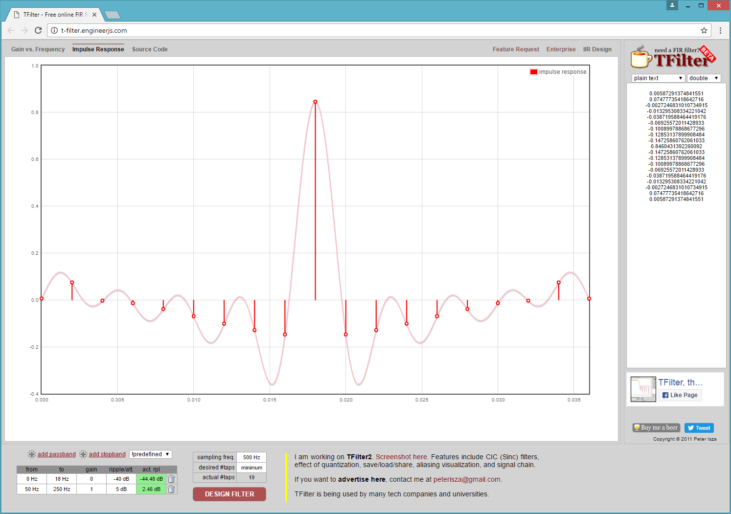
With time running out, it's time to pull together all that has been learned up to now, get the Java code ready to port to C/C++ and implement real filters as opposed to using running averages. In runF6(), I had been pulling together the theory that I need to filter out the bias on the front end with a high pass filter and then try to use a low pass filter on the remaining signal to find bursts of acceleration that occur at a 2 to 4 Hertz frequency. No way was I going to learn how to calculate my own filter tap values to implement the high and low pass filters in the small amount of time left before the deadline. Luckily, I discovered the t-filter web site. Talk about a triple play. Not only was I able to put in my parameters and get filter tap values, I was also able to leverage the C code it generated with a few tweaks in my Java code. Plus, it converted the tap values to fixed point for me! Fully employing the divide and conquer concept, this final version of the algorithm introduced isolated sub algorithms for both Front End Processor and Detection Processing. This allowed me to isolate the two functions from each other except for the output signal of one becoming the input to the other, which enabled me to focus easily on the task at hand rather than sift through a large group of variables where some might be shared between the two stages.

With this division of responsibility, it is now easy to focus on making the clear task of the Front End Processor to remove the bias values and output at a level that is readily acceptable for input into the Detection Processor. Now the Detection processor can clearly focus on filtering and implementing a state machine that can pick out the punch events that should occur between 2 and 4 times per second.

One thing to note is that this final algorithm is much smaller and simpler than some of the previous algorithms. Even though its software, at some point in the process you should still do a technique called Muntzing. Muntzing is a technique to go back and look at what can be removed without breaking the functionality. Every line of code that is removed is one less line of code that can have a bug. You can Google Earl “Madman” Muntz to get a better understanding and feel for the spirit of Muntzing.

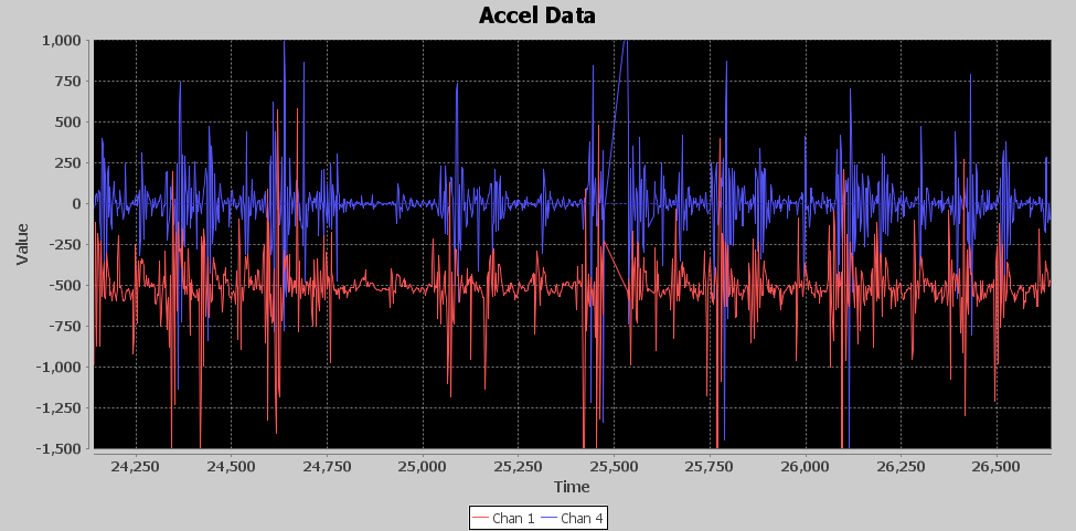
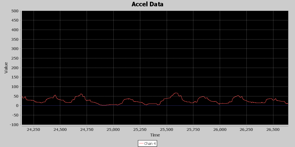
Above is the visual output from runF6. The Green line is 45 samples delayed of the output of the low pass filter, and the yellow line is an average of 99 values of the output of the low pass filter. The Detection Processor includes a detection algorithm that detects punches by tracking min and max crossings of the Green signal using the Yellow signal as a template for dynamic thresholding. Each minimum is a Red spike, and each maximum is a Blue spike, which is also a punch detection. The timescale is in milliseconds. Notice there are about three blue spikes per second inside the 2 to 4Hz range predicted. And the rest is history!

Algorithm Components

Here is a brief look at each type of component I used in the various algorithms.

Delay

This is used to buffer a signal so you can time align it to some other operation. For example, if you average nine samples and you want to subtract the average from the original signal, you can use a delay of five samples of the original signal so you can use values that are itself plus the four samples before and four samples after.

Attenuate

Attenuation is a simple but useful operation that can scale a signal down before it is amplified in some fashion with filtering or some other operation that adds gain to the signal. Typically attenuation is measured in decibels (dB). You can attenuate power or amplitude depending on your application. If you cut the amplitude by half, you are reducing it by -6 dB. If you want to attenuate by other dB values, you can check the dB scale here. As it relates to the Speedbag algorithm, I’m basically trying to create clear gaps in the signal, for instance squelching or squishing smaller values closer to zero so that squaring values later can really push the peaks higher but not having as much effect on the values pushed down towards zero. I used this technique to help accentuate the bursts of acceleration versus background vibrations of the speed bag platform.

Sliding Window Average

Sliding Window Average is a technique of calculating a continuous average of the incoming signal over a given window of samples. The number of samples to be averaged is known as the window size. The way I like to implement a sliding window is to keep a running total of the samples and a ring buffer to keep track of the values. Once the ring buffer is full, the oldest value is removed and replaced with the next incoming value, and the value removed from the ring buffer is subtracted from the new value. That result is added to the running tally. Then simply divide the running total by the window size to get the current average whenever needed.

Rectify

This is a very simple concept which is to change the sign of the values to all positive or all negative so they are additive. In this case, I used rectification to change all values to positive. As with rectification, you can use a full wave or half wave method. You can easily do full wave by using the abs() math function that returns the value as positive. You can square values to turn them positive, but you are changing the amplitude. A simple rectify can turn them positive without any other effects. To perform half wave rectification, you can just set any value less than zero to zero.

Compression

In the DSP world Compression is typically defined as compressing the amplitudes to keep them in a close range. My compression technique here is to sum up the values in a window of samples. This is a form of down-sampling as you only get one sample out each time the window is filled, but no values are being thrown away. It’s a pure total of the window, or optionally an average of the window. This was employed in a few of the algorithms to try to identify bursts of acceleration from quieter times. I didn’t actually use it in the final algorithm.

FIR Filter

Finite Impulse Response (FIR) is a digital filter that is implemented via a number of taps, each with its assigned polynomial coefficient. The number of taps is known as the filter’s order. One strength of the FIR is that it does not use any feedback, so any rounding errors are not cumulative and will not grow larger over time. A finite impulse response simply means that if you input a stream of samples that consisted of a one followed by all zeros, the output of the filter would go to zero within at most the order +1 amount of 0 value samples being fed in. So, the response to that single sample of one lives for a finite amount of samples and is gone. This is essentially achieved by the fact there isn’t any feedback employed. I’ve seen DSP articles claim calculating filter tap size and coefficients is simple, but not to me. I ended up finding an online app called tFilter that saved me a lot of time and aggravation. You pick the type of filter (low, high, bandpass, bandstop, etc) and then setup your frequency ranges and sampling frequency of your input data. You can even pick your coefficients to be produced in fixed point to avoid using floating point math. If you're not sure how to use fixed point or never heard of it, I’ll talk about that in the Embedded Optimization Techniques section.

Embedded Optimization Techniques

Magnitude Squared

Mag Square is a technique that can save computing power of calculating square roots. For example, if you want to calculate the vector for X and Z axis, normally you would do the following: val = sqr((X * X) + (Y * Y)). However, you can simply leave the value in (X * X) + (Y * Y), unless you really need the exact vector value, the Mag Square gives you a usable ratio compared to other vectors calculated on subsequent samples. The numbers will be much larger, and you may want to use attenuation to make them smaller to avoid overflow from additional computation downstream.

I used this technique in the final algorithm to help accentuate the bursts of acceleration from the background vibrations. I only used Z * Z in my calculation, but I then attenuated all the values by half or -6dB to bring them back down to reasonable levels for further processing. For example, after removing the bias if I had some samples around 2 and then some around 10, when I squared those values I now have 4 and 100, a 25 to 1 ratio. Now, if I attenuate by .5, I have 2 and 50, still a 25 to 1 ratio but now with smaller numbers to work with.

Fixed Point

Using fixed point numbers is another way to stretch performance, especially on microcontrollers. Fixed point is basically integer math, but it can keep precision via an implied fixed decimal point at a particular bit position in all integers. In the case of my FIR filter, I instructed tFilter to generate polynomial values in 16-bit fixed point values. My motivation for this was to ensure I don’t use more than 32-bit integers, which would especially hurt performance on an 8-bit microcontroller.

Rather than go into the FIR filter code to explain how fixed point works, let me first use a simple example. While the FIR filter algorithm does complex filtering with many polynomials, we could implement a simple filter that outputs the same input signal but -6dB down or half its amplitude. In floating point terms, this would be a simple one tap filter to multiply each incoming sample by 0.5. To do this in fixed point with 16 bit precision, we would need to convert 0.5 into its 16-bit fixed point representation. A value of 1.0 is represented by 1 * (2^16) or 65,536. Anything less than 65536 is a value less than 1. To create a fixed point integer of 0.5, we simply use the same formula 0.5 * (2^16), which equals 32,768. Now we can use that value to lower the amplitude by .5 of every sample input. For example, say we input into our simple filter a sample with the value of 10. The filter would calculate 10 * 32768 = 327,680, which is the fixed point representation. If we no longer care about preserving the precision after the calculations are performed, it can easily be turned back into a non-fixed point integer by simply right shifting by the number of bits of precision being used. Thus, 327680 >> 16 = 5. As you can see, our filter changed 10 into 5 which of course is the one half or -6dB we wanted out. I know 0.5 was pretty simple, but if you had wanted 1/8 the amplitude, the same process would be used, 65536 * .125 = 8192. If we input a sample of 16, then 16 * 8192 = 131072, now change it back to an integer 131072 >> 16 = 2. Just to demonstrate how you lose the precision when turning back to integer (the same as going float to integer) if we input 10 into the 1/8th filter it would yield the following, 10 * 8192 = 81920 and then turning it back to integer would be 81920 >> 16 = 1, notice it was 1.25 in fixed point representation.

Getting back to the FIR filters, I picked 16 bits of precision, so I could have a fair amount of precision but balanced with a reasonable amount of whole numbers. Normally, a signed 32-bit integer can have a range of - 2,147,483,648 to +2,147,483,647, however there now are only 16 bits of whole numbers allowed which is a range of -32,768 to +32,767. Since you are now limited in the range of numbers you can use, you need to be cognizant of the values being fed in. If you look at the FEPFilter_get function, you will see there is an accumulator variable accZ which sums the values from each of the taps. Usually if your tap history values are 32 bit, you make your accumulator 64-bit to be sure you can hold the sum of all tap values. However, you can use a 32 bit value if you ensure that your input values are all less than some maximum. One way to calculate your maximum input value is to sum up the absolute values of the coefficients and divide by the maximum integer portion of the fixed point scheme. In the case of the FEP FIR filter, the sum of coefficients was 131646, so if the numbers can be 15 bits of positive whole numbers + 16 bits of fractional numbers, I can use the formula (2^31)/131646 which gives the FEP maximum input value of + or - 16,312. In this case, another optimization can be realized which is not to have a microcontroller do 64-bit calculations.

Walking the Signal Processing Chain

Delays Due to Filtering

Before walking through the processing chain, we should discuss delays caused by filtering. Many types of filtering add delays to the signal being processed. If you do a lot of filtering work, you are probably well aware of this fact, but, if you are not all that experienced with filtering signals, it’s something of which you should be aware. What do I mean by delay? This simply means that if I put in a value X and I get out a value Y, how long it takes for the most impact of X to show up in Y is the delay. In the case of a FIR filter, it can be easily seen by the filter’s Impulse response plot, which, if you remember from my description of FIR filters, is a stream of 0’s with a single 1 inserted. T-Filter shows the impulse response, so you can see how X impacts Y’s output. Below is an image of the FEP’s high pass filter Impulse Response taken from the T-Filter website. Notice in the image that the maximum impact on X is exactly in the middle, and there is a point for each tap in the filter.

Below is a diagram of a few of the FEP’s high pass filter signals. The red signal is the input from the accelerometer or the newest sample going into the filter, the blue signal is the oldest sample in the filter’s ring buffer. There are 19 taps in the FIR filter so they represent a plot of the first and last samples in the filter window. The green signal is the value coming out of the high pass filter. So to relate to my X and Y analogy above, the red signal is X and the green signal is Y. The blue signal is delayed by 36 milliseconds in relation to the red input signal which is exactly 18 samples at 2 milliseconds, this is the window of data that the filter works on and is the Finite amount of time X affects Y.

Notice the output of the high pass filter (green signal) seems to track changes from the input at a delay of 18 milliseconds, which is 9 samples at 2 milliseconds each. So, the most impact from the input signal is seen in the middle of the filter window, which also coincides with the Impulse Response plot where the strongest effects of the 1 value input are seen at the center of the filter window.

It’s not only a FIR that adds delay. Usually, any filtering that is done on a window of samples will cause a delay, and, typically, it will be half the window length. Depending on your application, this delay may or may not have to be accounted for in your design. However, if you want to line this signal up with another unfiltered or less filtered signal, you are going to have to account for it and align it with the use of a delay component.

Front End Processor

I’ve talked at length about how to get to a final solution and all the components that made up the solution, so now let’s walk through the processing chain and see how the signal is transformed into one that reveals the punches. The FEP’s main goal is to remove bias and create an output signal that smears across the bursts of acceleration to create a wave that is higher in amplitude during increased acceleration and lower amplitude during times of less acceleration. There are four serial components to the FEP: a High Pass FIR, Attenuator, Rectifier and Smoothing via Sliding Window Average.

The first image is the input and output of the High Pass FIR. Since they are offset by the amount of bias, they don’t overlay very much. The red signal is the input from the accelerometer, and the blue is the output from the FIR. Notice the 1g of acceleration due to gravity is removed and slower changes in the signal are filtered out. If you look between 24,750 and 25,000 milliseconds, you can see the blue signal is more like a straight line with spikes and a slight ringing on it, while the original input has those spikes but meandering on some slow ripple.

Next is the output of the attenuator. While this component works on the entire signal, it lowers the peak values of the signal, but its most important job is to squish the quieter parts of the signal closer to zero values. The image below shows the output of the attenuator, and the input was the output of the High Pass FIR. As expected, peaks are much lower but so is the quieter time. This makes it a little easier to see the acceleration bursts.

Next is the rectifier component. Its job is to turn all the acceleration energy in the positive direction so that it can be used in averaging. For example, an acceleration causing a positive spike of 1000 followed by a negative spike of 990 would yield an average of 5, while a 1000 followed by a positive of 990 would yield an average of 995, a huge difference. Below is an image of the Rectifier output. The bursts of acceleration are slightly more visually apparent, but not easily discernable. In fact, this image shows exactly why this problem is such a tough one to solve; you can clearly see how resonant shaking of the base causes the pattern to change during punch energy being added. The left side is lower and more frequent peaks, the right side has higher but less frequent peaks.

The 49 value sliding window is the final step in the FEP. While we have done subtle changes to the signal that haven’t exactly made the punches jump out in the images, this final stage makes it visually apparent that the signal is well on its way of yielding the hidden punch information. The fruits of the previous signal processing magically show up at this stage. Below is an image of the Sliding Window average. The blue signal is its input or the output of the Rectifier, and the red signal is the output of the sliding window. The red signal is also the final output of the FEP stage of processing. Since it is a window, it has a delay associated with it. Its approximately 22 samples or 44 milliseconds on average. It doesn’t always look that way because sometimes the input signal spikes are suddenly tall with smaller ringing afterwards. Other times there are some small spikes leading up to the tall spikes and that makes the sliding window average output appear inconsistent in its delay based on where the peak of the output shows up. Although these bumps are small, they are now representing where new acceleration energy is being introduced due to punches.

Detection Processor

Now it’s time to move on to the Detection Processor (DET). The FEP outputs a signal that is starting to show where the bursts of acceleration are occurring. The DET’s job will be to enhance this signal and employ an algorithm to detect where the punches are occurring.

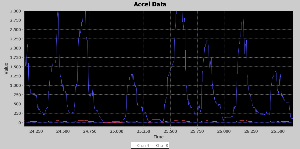
The first stage of the DET is an attenuator. Eventually, I want to add exponential gain to the signal to really pull up the peaks, but, before doing that, it is important to once again squish down the lower values towards zero and lower the peaks to keep from generating values too large to process in the rest of the DET chain. Below is an image of the output from the attenuator stage, it looks just like the signal output from the FEP, however notice the signal level peaks were above 100 from the FEP, and now peaks are barely over 50. The vertical scale is zoomed in with the max amplitude set to 500 so you can see that there is a viable signal with punch information.

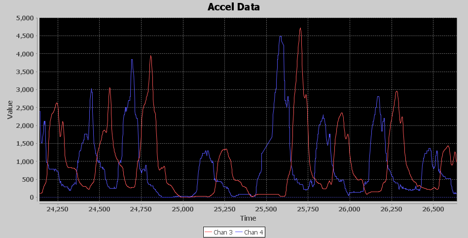
With the signal sufficiently attenuated, it’s time to create the magic. The Magnitude Square function is where it all comes together. The attenuated signal carries the tiny seeds from which I’ll grow towering Redwoods. Below is an image of the Mag Square output, the red signal is the attenuated input, and the blue signal is the mag square output. I’ve had to zoom out to a 3,000 max vertical, and, as you can see, the input signal almost looks flat, yet the mag square was able to pull out unmistakable peaks that will aid the detection algorithm to pick out punches. You might ask why not just use these giant peaks to detect punches. One of the reasons I’ve picked this area of the signal to analyze is to show you how the amount of acceleration can vary greatly as you can see the peak between 25,000 and 25,250 is much smaller than the surrounding peaks, which makes pure thresholding a tough chore.

Next, I decided to put a Low Pass filter to try to remove any fast changing parts of the signal since I’m looking for events that occur in the 2 to 4 Hz range. It was tough on T-Filter to create a tight low pass filter with a 0 to 5 Hz band pass as it was generating filters with over 100 taps, and I didn’t want to take that processing hit, not to mention I would then need a 64-bit accumulator to hold the sum. I relaxed the band pass with a 0 to 19 Hz range and the band stop at 100 to 250 Hz. Below is an image of the low pass filter output. The blue signal is the input, and the red signal is the delayed output. I used this image because it allows the input and output signal to be seen without interfering with each other. The delay is due to 6 sample delay of the low pass FIR, but I have also introduced a 49 sample delay to this signal so that it is aligned in the center of the 99 sample sliding window average that follows in the processing chain. So it is delayed by a total of 55 samples or 110 milliseconds. In this image, you can see the slight amplification of the slow peaks by their height and how it is smoothed as the faster changing elements are attenuated. Not a lot going on here but the signal is a little cleaner, Earl Muntz might suggest I cut the low pass filter out of the circuit, and it might very well work without it.

The final stage of the signal processing is a 99 sample sliding window average. I built into the sliding window average the ability to return the sample in the middle of the window each time a new value is added and that is how I produced the 49 sample delayed signal in the previous image. This is important because the detection algorithm is going to have 2 parallel signals passed into it, the output of the 99 sliding window average and the 49 sample delayed input into the sliding window average. This will perfectly align the un-averaged signal in the middle of the sliding window average. The averaged signal is used as a dynamic threshold for the detection algorithm to use in its detection processing. Here, once again, is the image of the final output from the DET.

In the image, the green and yellow signals are inputs to the detection algorithm, and the blue and red are outputs. As you can see, the green signal, which is a 49 samples delayed, is aligned perfectly with the yellow 99 sliding window average peaks. The detection algorithm monitors the crossing of the yellow by the green signal. This is accomplished by both maximum and minimum start guard state that verifies the signal has moved enough in the minimum or maximum direction in relation to the yellow signal and then switches to a state that monitors the green signal for enough change in direction to declare a maximum or minimum. When the peak start occurs and it’s been at least 260ms since the last detected peak, the state switches to monitor for a new peak in the green signal and also makes the blue spike seen in the image. This is when a punch count is registered. Once a new peak has been detected, the state changes to look for the start of a new minimum. Now, if the green signal falls below the yellow by a delta of 50, the state changes to look for a new minimum of the green signal. Once the green signal minimum is declared, the state changes to start looking for the start of a new peak of the green signal, and a red spike is shown on the image when this occurs.

Again, I’ve picked this time in the recorded data because it shows how the algorithm can track the punches even during big swings in peak amplitude. What’s interesting here is if you look between the 24,750 and 25,000 time frame, you can see the red spike detected a minimum due to the little spike upward of the green signal, which means the state machine started to look for the next start of peak at that point. However, the green signal never crossed the yellow line, so the start of peak state rode the signal all the way down to the floor and waited until the cross of the yellow line just before the 25,250 mark to declare the next start of peak. Additionally, the peak at the 25,250 mark is much lower than the surrounding peaks, but it was still easily detected. Thus, the dynamic thresholding and the state machine logic allows the speed bag punch detector algorithm to “Roll with the Punches”, so to speak.

Final Thoughts

To sum up, we’ve covered a lot of ground in this article. First, the importance of fully understanding the problem as it relates to the required end item along with the domain knowledge needed to get there. Second, for a problem of this nature creating a scaffold environment to build the algorithm was imperative, and in this instance, it was the Java prototype with visual display of the signals. Third, was implement for the target environment, on a PC you have wonderful optimizing compilers for powerful CPUs with tons of cache, for a microcontroller the optimization is really left to you. Use every optimization trick you know to keep processing as quick as possible. Fourth, iterative development can help you on problems like this. Keep reworking the problem while folding in the knowledge you are learning during the development process.

When I look back on this project and think about what ultimately made me successful, I can think of two main things. Creating the right tools for the job was invaluable. Being able to see how my processing components were affecting the signal was really invaluable. Not only plotting the output signal, but having it plot in realtime, allowed me to fully understand the acceleration being generated. It was as if Nate was in the corner punching the bag, and I was watching the waveform roll in on my screen. However, the biggest factor was realizing that in the end I am looking for something that happens 2 to 4 times per second. I latched on to that and relentlessly pursued how to translate the raw incoming signal into something that would show those events. There was nothing for me to Google to find that answer. Remember knowledge doesn’t really come from books, it gets recorded in books. First, someone had to go off script and discover something and then it becomes knowledge. Apply the knowledge you have and can find, but don’t be afraid to use your imagination to try what hasn’t been tried before to solve an unsolved problem. So remember in the future, metaphorically when you come to the end of the paved road. Will you turn around looking for a road already paved ,or will you lock in the hubs and keep plowing ahead to make your own discovery. I wasn’t able to just Google how to count punches with an accelerometer, but now someone can.

For more informational fun, check out these other great SparkFun write-ups.