Programming FPGAs: Papilio Pro

Contributors: Toni_K

Basic Simulation using PlanAhead

Now that we know the basics of HDL, let's get into the project of this tutorial.

A few notes on the project:

• The project itself DOES NOT MEET TIMING. This is due to the clock domain conversion being performed within the program.
• The project already contains an existing bitstream.
• I tried to comment as much as possible, while keeping it from being a novel. If you have any questions, please post in the comments section.

Simulation is a key part of the FPGA design process. Unlike microcontroller development, we want to make sure the code we have written functions the way we want it to before pushing it to the chip. Some microcontroller development software provide their own simulation, but in the open source arena, I have not seen this.

So why MUST we simulate before we go further?

1. Compilation takes time and a lot of resources (depending on the design). It is not wise to go through this flow for every little change in the design.
2. FPGAs by definition are not cheap parts (unless you buy in bulk). An incorrect design does have a slim chance on damaging the board, chip, or both.
3. We can find bugs in the code earlier and fix them without even compiling the code, which makes things faster.

These are my top three answers. Others might agree/disagree, but that is the beauty of engineering.

How to Run the Code

Once you have installed the program files, open up PlanAhead, and select "Create New Project". Choose the path where you would like your project to be located. You can then navigate to the source files you downloaded previously. Choose the "Spartan 6" as the Family and the "XC6SLX9tqg144-2" as the Project Part.

How to Stimulate the Code

Writing stimulus for simulation is fairly easy and by far one of the more creative aspects of FPGA designs. The reason is, you get to find ways to break the design in the fewest lines of code.

Here is the stimulus for the clock divider (clk_div_tb.v) in the previous sections:

`timescale 1ns / 1ps

module clk_div_tb();

reg clk_in;
reg rst;
reg ce;

wire [nDelay-1:0] clk_out;

parameter nDelay = 32;

genvar i;
generate
   for(i = 0; i < nDelay; i = i + 1) begin
      clk_div #(
         .DELAY(i)
      ) DUT (
         .clk_in(clk_in), 
         .rst(rst), 
         .ce(ce), 
         .clk_out(clk_out[i])
      );
   end
endgenerate

always #15.625 clk_in = ~clk_in;

// Initial input states
initial begin
   clk_in = 0;
   rst = 1;
   ce = 1;
end

// Test procedure below
initial begin
   #100 rst = 0;

end

endmodule

Let's break down the code.

1. The stimulus (test bench) is considered a module ON TOP of the module in test. In this case clk_div_tb is the top-level of clk_div.
2. Inputs are always reg and outputs are always wires. The reason is, you manipulate the inputs and it has to process through the system to the outputs. (We will be able to tap into the design's internal wires.)
3. We are generating clock dividers on purpose here. The generate block lets us do multiple instantiations of the clk_div instance. The genvar is the variable we use in the for-loop to keep things consistent (think of this as doing an int i for C++ and then using the i as the loop variable.
   • The reason we are generating 32 of these is because, at the time I was not sure which delay value was going to be the best. By doing it this way, I could easily check which delay value would be best.
4. The always block is basically saying, "clk_in is going to be going from logic low/high to high/low (depending on the reset state of clk_in". The value #15.625 is used because that is matching the frequency that is used by the Papilio Pro.
5. Next is the initial values. All inputs will have initial values. This is why we always design with a reset state in mind. Here, clk_in is logic low, rst and ce are logic high.
6. We add our stimulus in the test procedure block. Here, we see that after #100 we set our rst to logic low. (This means our reset is active high). The #100 dignifies how many time units it'll be from the start 'til rst's value changes.
   • If you wanted to add stimulus to this after the reset, you could. As an example, you can put: #150 ce = 0;. This means, after 50 clock pulses, make the ce signal GND, or basically turn off this submodule.

See the timescale 1ns/1ps at the top? This tells the simulator the unit value of # and the resolution. In this case, 1ns is our unit of time, and 1ps is our resolution. This is extremely detailed for our design, but it works since we are working with a 32MHz clock frequency.

Running the Simulation

In PlanAhead, running a simulation is quite easy.

In the Flow navigator, there's a button that says Run Behavioral Simulation. Press this button, and a dialog will appear. This is where we can select a simulation set and the top-level simulation to use, as well as options for the simulation itself. Generally, the options should be kept at default. Now, the top module name we see is not what we want. Click the button that looks like ..., and it'll bring up a window with a selection of what PlanAhead believes to be simulation test benches. Most engineers will label their simulation files by appending them with a _tb. This helps them identify what is the design and what is not. For us, let us select the clk_div_tb. This will test our clock divider module.

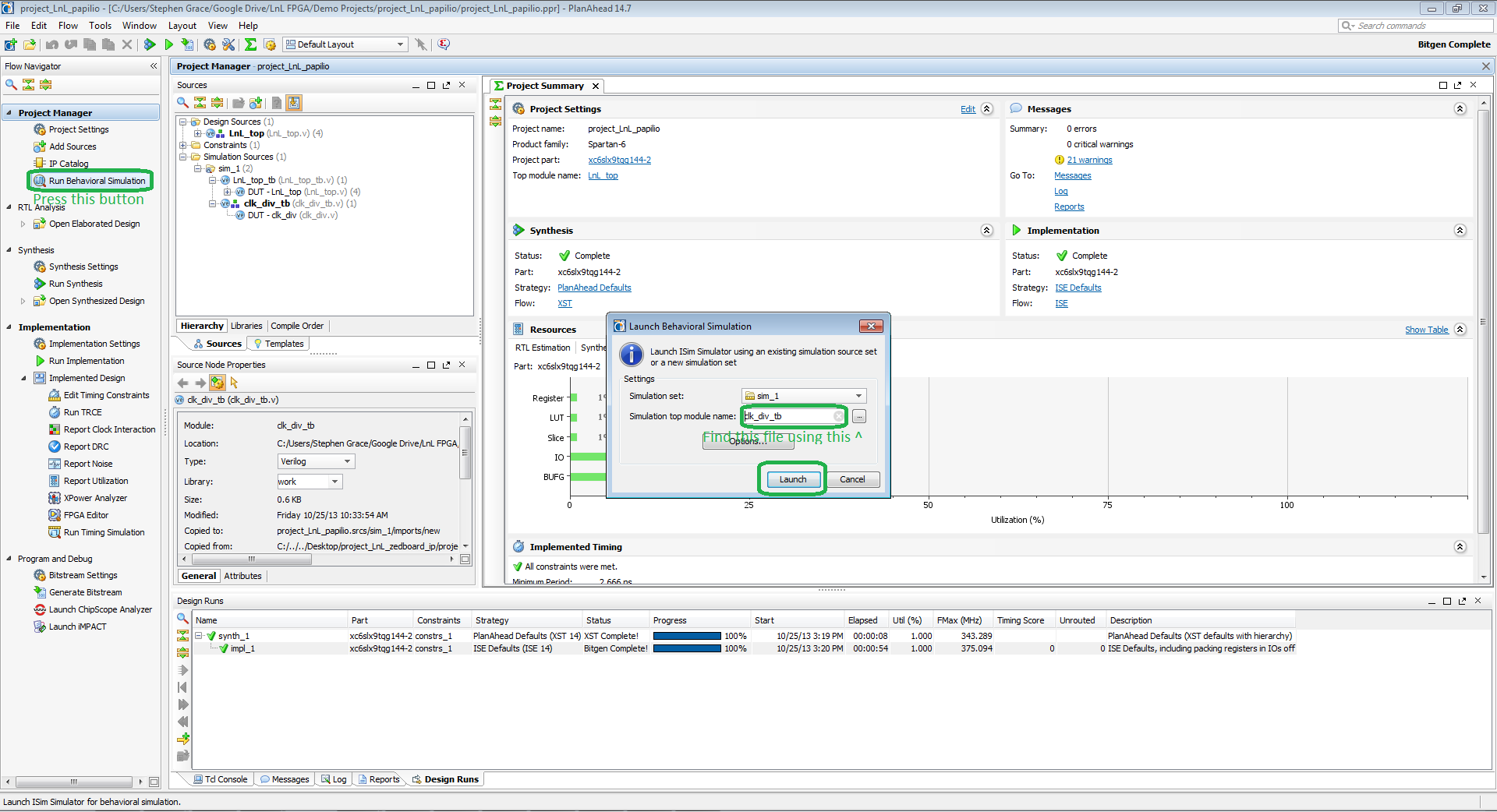
Click Launch. This will launch the ISim software provided and run the test. By default, it'll run for 5microseconds, and, for the purpose of this tutorial, that is long enough. Wait for it finish, and then we'll look at the waveforms.

Understanding the Waveforms

Waveforms is a set of signals that we determine to be important enough to warrant us viewing them and analyzing the fine timing of positive and negative edge changes.

NOTE: Simulations use "ideal" switching. This means that they are GND and VCC at the same time in the viewer. In reality, this is not true.

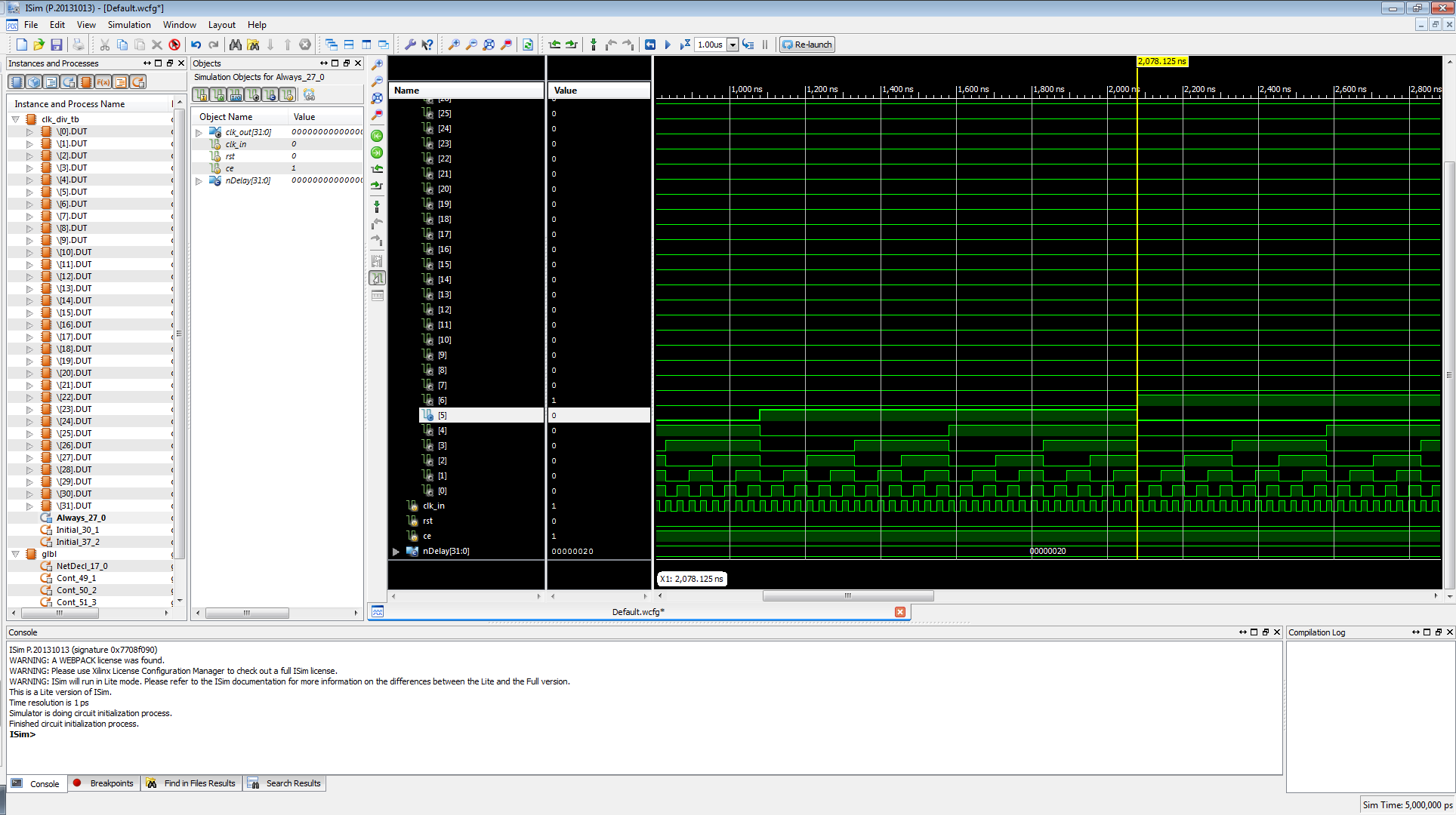
Here is the waveform window we see after the simulation:

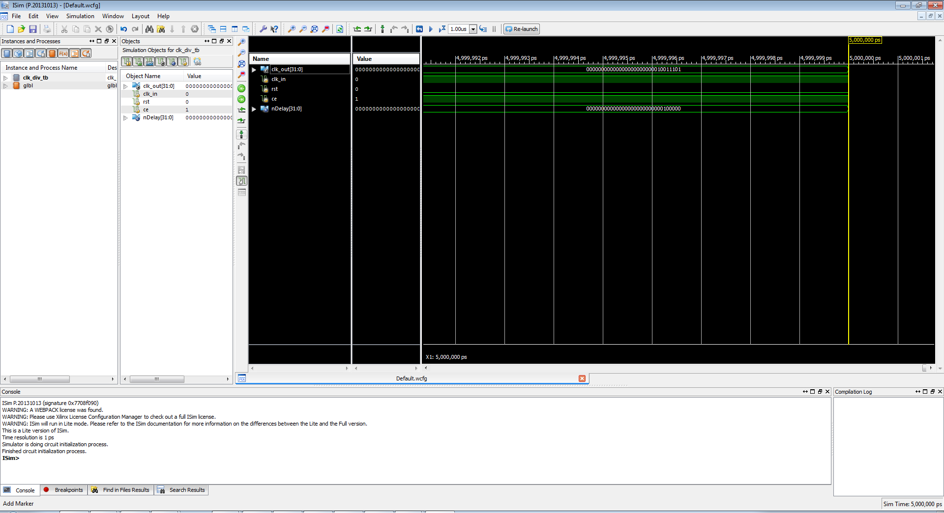
The view can be very complex, but what we're interested in is where all the green and black is.

This is the waveforms of the clock divider. If you look back at the code, I have nDelay set to 32, and if we look at the waveform, we see clk_out as clk_out[31:0] and nDelay as nDelay[31:0]. Generally, the waveform viewer is showing all 32 bits in binary. This is not helpful for anyone, and since we know hex, let's change it to that.

To change the radix to hex, select clk_out and nDelay in the view (Ctrl+Click each signal in the view). In the Value column, right-click, go to the Radix submenu, and select hexadecimal.

This is easier to read.

Let's expand the clk_out signal to look at all 32 signals.

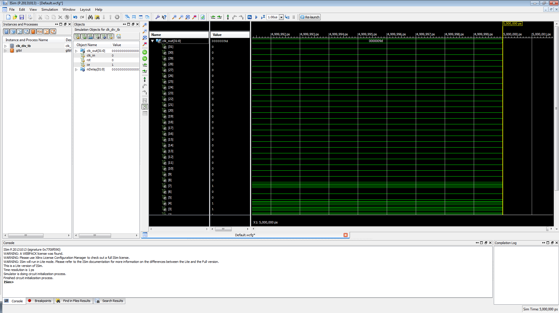
If you scroll down, you notice that we're only looking at 5 million picoseconds. That resolution is far too high, let's fix this. To change the view right-click on where the signals are, and click "To Full View".

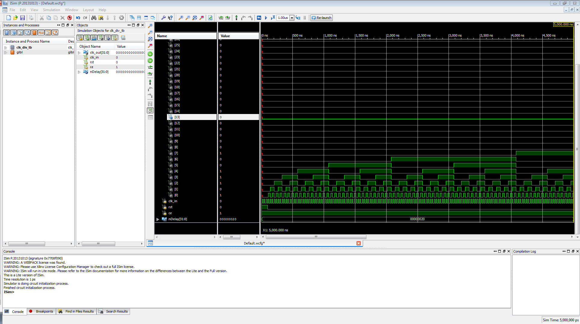
Now we can see far more info that is very useful and relevant for us.

Here we can do a couple things:

1. We can analyze the signals to see if they meet the proper timing arcs.
2. Check to see if the delay values we've added would work.

For this tutorial, let's just do #2, because #1 takes some advanced timing knowledge that is not necessary here.

This viewer has the ability to add markers to the waveforms, which will allow us to figure out how fast signals are and if they are within the timing arcs we want.

Firstly, select clk_out[5] signal. Notice how it goes bold green. Now let's check to see what frequency it is on. Remember, Frequency is the inverse of time elapsed, and 1Hz is 1 cycle. For this cycle, we are going to do a positive rising edge to positive rising edge.

To get this info, find the 2nd positive rising edge of clk_out[5], and click and drag from that point to the 1st positive rising edge. You should get the data in the screenshot.

Don't get too frustrated if you don't get it at first, most people eyeball it. Now we have the info we want.

To determine frequency from the two time values, we will just typically subtract, and the data we get is 2000ns. If you look closely in the screenshot, at the bottom, where it has a DeltaX, we see -2000ns. (Don't worry about the negative, that just means we're using the 2nd positive rising edge as the origin.)

Frequency = 1 / time -->, F = 1/(2000ns), and if you click here, you will see Google tell us 500kHz.

So, with a delay of 6 registers, we get 500kHz. For the 5microseconds test, try it with others and see what values you can get.

Did you notice a pattern? For each additional register we add, the delay increases by 2x. Meaning, if you did the clk_out[4] you would see 1000kHz (1MHz).

Pretty slick, huh?

Now let's make sure the signals, falling edges on clk_out[5], and clk_out[4] are in sync. Go ahead and select one of the falling edges for clk_out[5], and you will notice that it is in sync with other signals. This is a good thing, because it means things are in working order and timing is met properly. If it was not meeting timing properly, signals would be skewed, and using the skill we learned above, could determine the difference to figure out if it is meeting timing constraints (setup/hold) or not.

Now that I've shown you some basics, go ahead and close the simulator. It will ask you if you want to save the .wcfg file. This basically means the next time you run this simulation, it'll display the waveforms this way. Go ahead and save it.

To explore a bit further, I suggest modifying the clk_div_tb.v by adding #150 ce = 0; below the #100 rst = 0; , saving the file, running another simulation, and seeing what happens.

From here on, it only gets more advanced, and I recommend watching videos, and reading articles on ISim to understand it better.