$259.95
In the previous tutorial, we showed you how to calculate the location of a sound using the new SparkX Qwiic Sound Trigger and the u-blox ZED-F9P GNSS receiver.
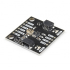
The Qwiic Sound Trigger can be used on its own, or as part of your Qwiic system. It is based on the VM1010 from Vesper Technologies and the TI PCA9536 GPIO expander. The VM1010 is a clever little device which can be placed into a very low power "Wake On Sound" mode. When it detects a sound, it wakes up and pulls its TRIG (DOUT) pin high. The VM1010 can then be placed into "Normal" mode by pulling the MODE pin low; it then functions as a regular microphone. The analog microphone signal is available on the AUDIO (VOUT) pin. All of this happens really quickly, within 50 microseconds (much faster than a capacitive MEMS microphone), so you don't miss the start of the audio signal. This makes it ideal for use as a sound trigger!
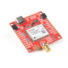
The u-blox ZED-F9P GNSS receiver is an old friend. It is a top-of-the-line module for high accuracy GNSS location solutions including RTK that is capable of 10mm, three-dimensional accuracy. With this board, you will be able to know where your (or any object's) X, Y, and Z location is within roughly the width of your fingernail! Something that doesn’t get discussed as much as it should is that the ZED-F9P can also capture the timing of a signal on its INT pin with nanosecond resolution! It does that through a UBX message called TIM_TM2.
In this tutorial, we take this to the next dimension. Quite literally! Last time, we used two sound trigger systems to calculate where a sound came from along the line from one trigger to the other. That’s a one-dimensional (1D) system. If we add a third sound trigger, we can triangulate the location of a sound in two dimensions (2D) allowing us to plot the position in X and Y or East and North!
Let's talk first about triangulation….
Last time, we learned that we can calculate the location of a sound by measuring the difference in the sound’s time-of-arrival at two sound triggers. In our 1D example, we:
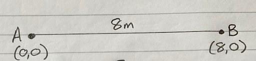
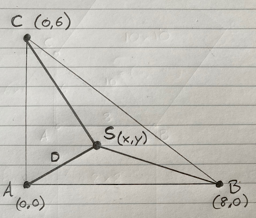
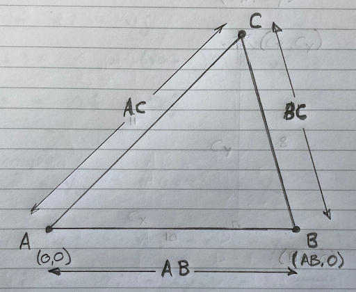
In 2D, there is a little more math involved. Let’s call our three sound trigger systems A, B and C. A is our reference or origin. If we position trigger B due East from A, we can call the line that joins A to B our X axis. Remember when you used to draw graphs in math class? You had the origin in the bottom left corner of your graph paper and you drew the X axis horizontally out to the right. We are doing the same thing here. Trigger A is our origin at X = 0 and Y = 0. We write that as (0,0). If Trigger B is 8 metres (8m) away from A, then its location is X = 8 and Y = 0. We write that as (8,0).
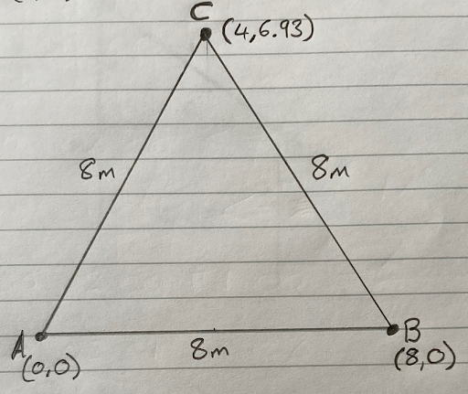
So far, so good. Now, where should we position trigger C? In reality, it doesn’t really matter. We could position C so that ABC forms a perfect equilateral triangle (a triangle where all three sides are the same length). That would give us the best coverage of the area. But the coordinates of C would be (4,6.93). Not pleasant.
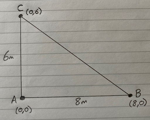
To keep the math simpler for this example, let’s position C 6m due North from A. The coordinates of C are X = 0 and Y = 6. We write that as (0,6).
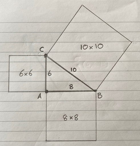
We know the distance from A to B is 8m, and that the distance from A to C is 6m. But what about the distance from B to C? We need to know that too. If we get out a tape measure and measure it, we’ll find it is exactly 10m. If you remember Pythagoras’ Theorem from your math class, the square on the hypotenuse is equal to the sum of the squares on the other two sides, we can calculate the distance from B to C by:
Again, to keep the math easier, let’s pretend that the speed of sound is 1 metre per second (1m/s), not 343.42m/s.
Now, let’s suppose our sound trigger system is running and it detects a sound:
Let’s calculate the differences in those times:
With the speed of sound being 1m/s, we now know that the sound travelled an extra 1.779614m when travelling to B compared to A. And we know that the sound travelled an extra 1.394449m when travelling to C compared to A.
What we do not know is how far the sound travelled to get to A. That’s the first thing we need to calculate.
Let’s call the location of the sound: S. Let’s call the coordinates of S: ( x , y ). Let’s call the distance from S to A: D.
If we sketch that - not to scale - it looks like this:
We know that:
In order to find the location of S, we need to use triangles. That’s why this technique is called “triangulation”. In trigonometry and geometry, triangulation is the process of determining the location of a point by forming triangles to it from known points.
If we divide our diagram up into more triangles:
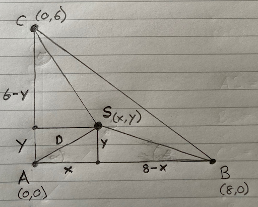
We can use Pythagoras’ Theorem to calculate the distances we need:
We can write that as:
We need to solve for D. To begin, let’s substitute the value for y2 from the second equation into the first equation:
Multiplying out the brackets, that becomes:
Simplifying, it becomes:
If we remove the brackets:
The D2 cancel out and so do the x2 leaving:
One final rearrange leaves:
If we divide through by 16 we are left with:
Now let’s go back to our three triangles:
This time, let’s substitute the value for x2 from the third equation into the first equation:
Multiplying out the brackets, that becomes:
If we remove the brackets:
Again, the D2 cancel out and so do the y2 leaving:
One final rearrange leaves:
If we divide through by 12 we are left with:
Now we can put our values for x and y back into our first equation:
D2 = x2 + y2
D2 = (-0.222452.D + 3.802061)2 + (-0.232408.D + 2.837959)2
Multiplying out the brackets, we get:
Simplifying:
Now, I’m sure you will remember quadratic equations from your math class too? We can solve for D using the equation:
( -b +/- √(b2 - 4.a.c ) ) / 2.a
a = 0.896502
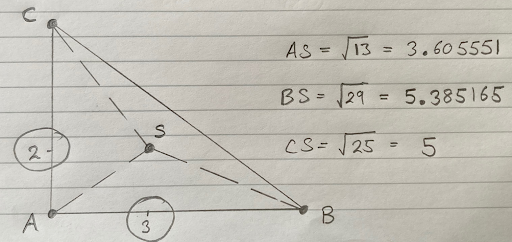
Inserting our values, D is:
Which equals:
We can ignore the negative value since it is not within our triangle. Now we know that D is 3.605550m !
Looking back at our equations for x and y:
If we insert the value for D, we can finally calculate the x and y coordinates of S:
Which is:
Fancy that!
This technique can be used on any configuration of trigger locations. They don’t have to be positioned in a neat right angle triangle. If you would like proof of that and would like to see the math to solve it, have a look at the section called Here There Be Dragons!
Thanks for sticking with us. The good news is that we’ve written more Python code to do that math for you!
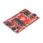
The GitHub Hardware Repo contains two examples for the Sound Trigger. You can run these in the Arduino IDE. The second example is the crowd pleaser! It runs on the MicroMod Data Logging Carrier Board together with the Artemis Processor Board but it should work just fine with any of our processor boards. It communicates with our ZED-F9P Breakout and the Qwiic Sound Trigger to capture sound events and log them to SD card as u-blox UBX TIM_TM2 messages.
Once you have your three sound event UBX TIM_TM2 files, our Sound_Trigger_Analyzer_2D.py will process the files for you and calculate the location of the sound events!
Run the Python code by calling:
language:python
python Sound_Trigger_Analyzer_2D.py TIM_TM2_A.ubx TIM_TM2_B.ubx TIM_TM2_C.ubx 8.0 6.0 10.0 20.0
The Python code will calculate and display the (x,y) coordinates of any valid sound events it finds. The coordinate system uses the location of A as the origin, and the line running from A to B as the X axis. The Y axis is (of course) 90 degrees counterclockwise from X.
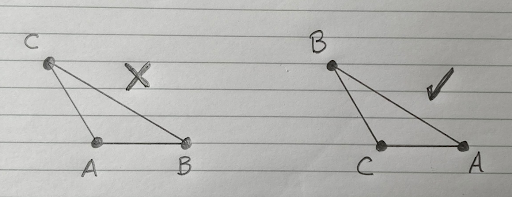
The calculation code assumes that the X coordinate of C is between A and B. If C lies to the left of A, or the right of B, then you need to rename your points. If C is to the left of A, then B becomes A, C becomes B, and A becomes C:
Enjoy your coordinates!
Sound_Trigger_Analyzer_2D.py can work with any configuration of the trigger positions (so long as the X coordinate of C is between A and B). They do not need to be arranged in a nice right-angled triangle with A-C pointing North. Don’t believe me? Want proof? Good for you! OK. Brace yourself. Here we go… Here is the actual math used in Sound_Trigger_Analyzer_2D.py.
Let’s suppose our three sound triggers are arranged such that they form a triangle ABC:
We know the length of the sides: AB, AC and BC.
We know the coordinates of A and B. A is our origin and is located at (0,0). B is due ‘East’ of A and defines our X axis. So we say that B is located at (AB,0). But we don’t yet know the location of C. We need to calculate it. Let’s call the location of C (CX,CY).
If we draw a line from C so it meets line A-B at right angles:
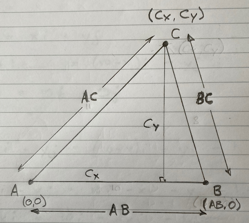
Pythagoras’ Theorem tells us that:
If we rearrange those equations, bringing CY2 to the left and multiplying out the brackets, we get:
Because those two equations are equal, we can arrange them as:
The two -CX2 cancel out. Rearranging, we get:
We can find CY by inserting the value for CX into one of our earlier equations:
So:
We now have the coordinates for C: ( CX , CY )
Now, let’s suppose our sound trigger system is running and it detects a sound. Let’s call the location of the sound S and give it coordinates ( SX , SY ):
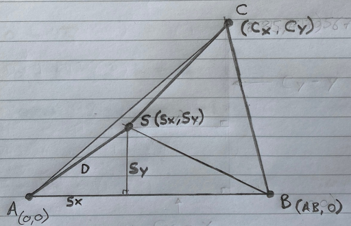
Our three systems are logging the time the sound arrives at each sensor (very accurately!).
The time taken for the sound to reach A is: the distance from S to A divided by the speed of sound. Likewise for B and C.
If all three systems hear the sound at the exact same time, then we know that the sound took an equal time to travel from S to A, B and C. That’s a special case where the distances SA, SB and SC are equal (equidistant). But usually sensors B and C will hear the sound at different times to A due to the distances SB and SC being different to SA. We need to include those differences in distance in our calculation. To save some typing, let’s call the distance SA: D
DdiffB is the difference between SB and D. Likewise, DdiffC is the difference between SC and D. Note that DdiffB or DdiffC could be negative if the source of the sound is closer to B or C than A.
Sensors B and C will hear the sound earlier or later than A depending on DdiffB and DdiffC.
What we do not know is how long the sound took to travel from S to A, because we do not know the distance D. That’s what we need to calculate,
What we do know is the difference in the time of arrival of the sound at our three sensors. If we bring the three sets of sensor data together, we can calculate the difference in the time of arrival at each sensor. Let’s say that:
Let’s calculate the differences in those times:
Again, TdiffB and TdiffC could be negative if the source of the sound is closer to B or C than A.
We can convert those differences in time into differences in distance by multiplying by the speed of sound:
Now we can use Pythogoras’ Theorem as before to study our triangles:
We need to add an extra triangle to include SC:
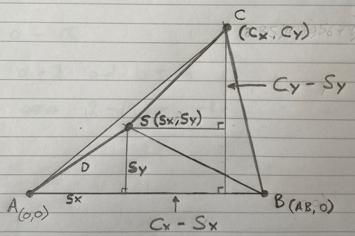
The width of the new triangle is:
The height of the new triangle is:
So, using Pythagoras’ Theorem again:
We now have our three equations:
We need to solve for D. To begin, let’s substitute the value for SY2 from the second equation into the first equation, so we can find the relationship between D and SX:
Multiplying out the brackets, that becomes:
As before, the D2 cancel and so do the SX2 leaving:
Rearranging:
Divide through by 2.AB:
Let’s make life easier for ourselves and say that:
Where:
We can calculate both values because we know AB and can calculate DdiffB:
Looking at equation 3 again:
If we replace SX with ( SXa.D + SXb ), we get:
Rearranging:
Multiplying out the bracket, it becomes:
Simplifying:
So:
That’s ever so slightly horrible, but let’s go with it…
Now we have values for SX and SY in terms of D, which we can plug into equation 5:
Substituting for SX and SY we get:
Multiplying out the brackets gives (brace yourself!):
Simplifying and moving everything but the root to the left gives:
Fortunately the D2 term cancels out completely, which is good news. If it didn’t, we’d have a quartic equation to solve instead of a quadratic…
Simplifying:
Dividing through by -2.CY gives:
We now need to square both sides to get rid of the root. Painful… But we need to do it… But first, to make life easier for ourselves, let’s simplify further and say:
Where:
Remember that we can already calculate values for da and db because we know or can calculate values for: DdiffC; CX; SXb; and CY.
Square both sides:
Moving the terms on the right over to the left:
That’s a quadratic equation which we can solve in the usual way. Let’s make:
Remember that we can already calculate values for qa, qb and qc because we already know: da; SXa; db; and SXb.
Solving the quadratic::
That gives us two possible values for D. One will be negative or otherwise invalid, leaving us with a value for D.
We can then plug the value for D into equation 6 to find the X coordinate of S because we already know the values of SXa and SXb:
We can then calculate the Y coordinate of S using equation 3:
Enjoy your coordinates!
learn.sparkfun.com | CC BY-SA 3.0 | SparkFun Electronics | Niwot, Colorado