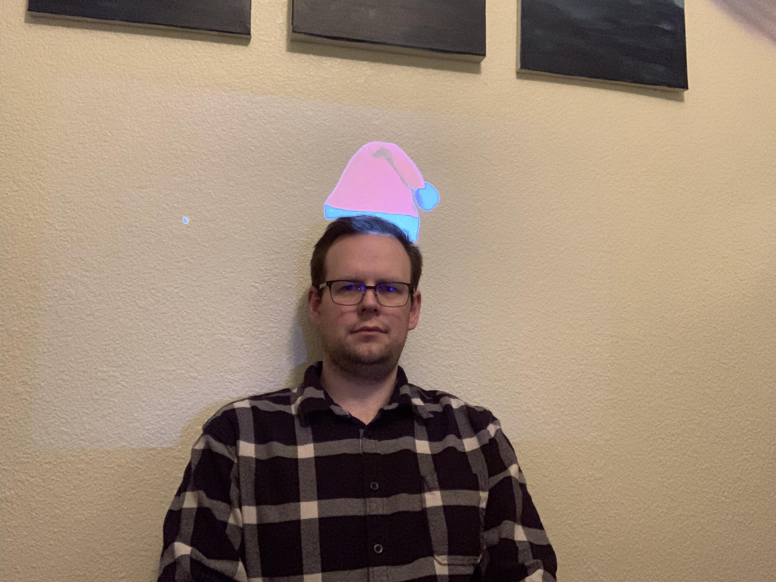
Let's face it - Python is pretty awesome, and what better way to make use of that awesomeness than to incorporate it into your projects? Here we're looking at some of the methods and libraries involved with projecting images using computer vision and Python. Since I’m finishing this tutorial around the holidays, it seems appropriate to create a Santa hat projector! Hopefully once you've completed the tutorial, you'll be able to substitute in whatever item you want for your own uses. To establish an acceptance criteria, I’ll consider this project finished when someone can walk in front of the projector and have the computer track them, projecting a Santa hat on their head.
To follow along with this tutorial, you will need the following materials. You may not need everything, depending on what you already have. Add it to your cart, read through the guide, and adjust the cart as necessary.
In addition you'll need:
We’ll start with a fresh install of Raspbian however you’d like to install it. There are lots of tutorials on how to do this, so I won’t go into it here (check out our tutorial).
Once the operating system is installed, we need to make sure that everything is up to date.
Open a terminal window and execute the following commands:
language:python
> sudo apt-get update
> sudo apt-get upgrade
> sudo apt-get dist-upgrade
This can take quite a while, depending on how out of date the software image you started with was.
The next part of computer vision is, well... the vision part. We’ll need to make sure that the PiCamera module is installed correctly.
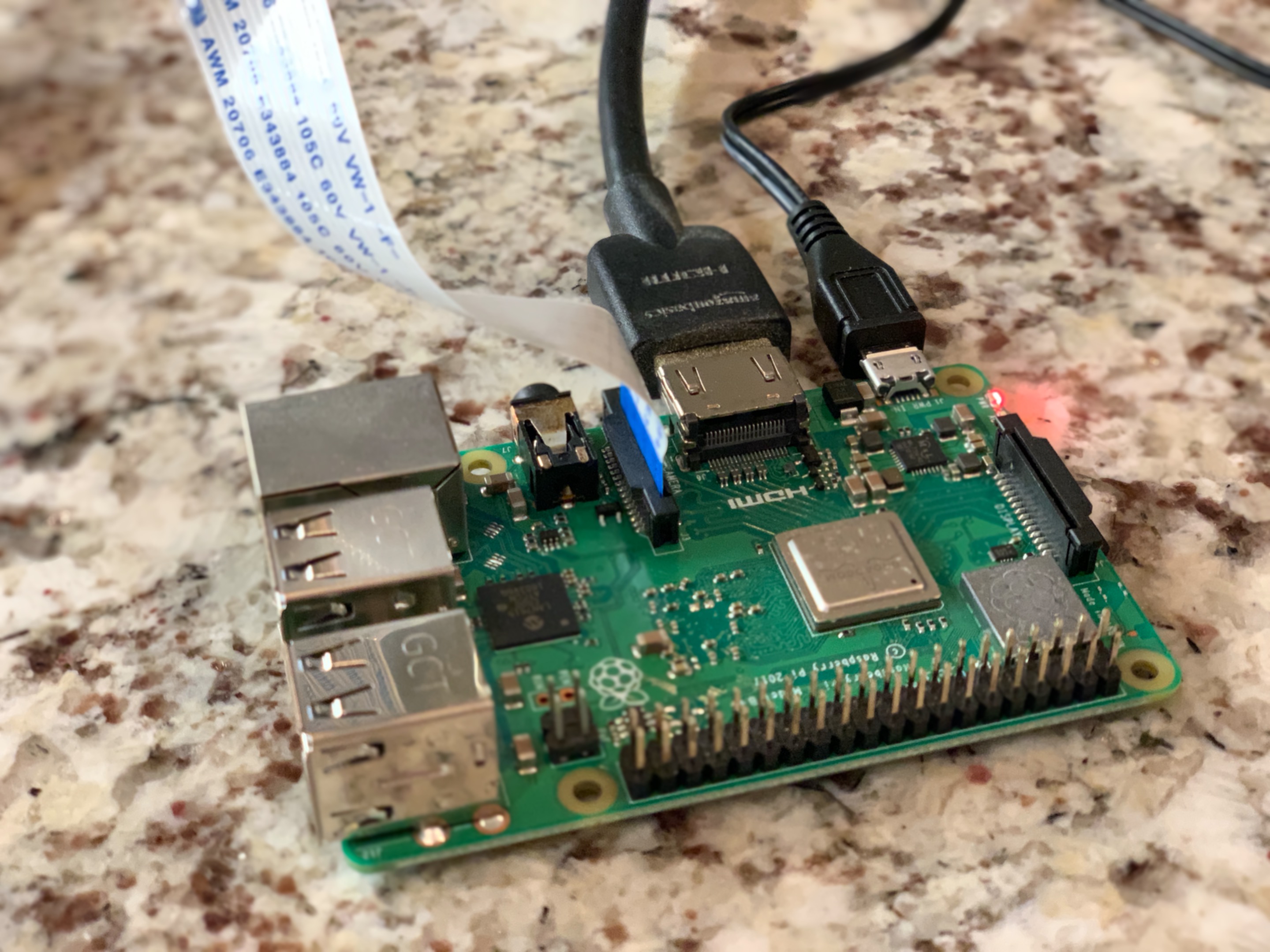
Start by making sure your Raspberry Pi is off, then open up the PiCamera module, and install it by inserting the cable into the Raspberry Pi. The camera connector is the one between the HDMI and Ethernet ports, and you’ll need to lift the connector clip before you can insert the cable. Install the cable with the silver contacts facing the HDMI port.
After you have the module physically installed, you’ll need to power on the Pi.
Launch the Raspberry Pi Config. There are two ways to do this, either from the command line, or from the desktop menu. Here’s the terminal command
language:python
> sudo raspi-config
You should see something like this
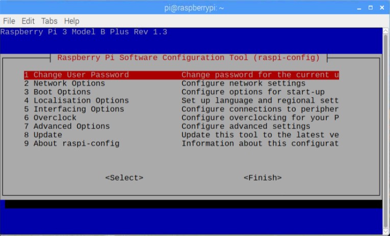
Under the Interfacing Options tab, enable the Camera module. You’ll need to reboot before the changes take effect. If you think you’ll use the features, it can be convenient to enable ssh and VNC while you’re at it. It should be noted that if you use VNC with some of the Pi Camera tutorials, some of the image preview windows don’t show up. If you are connected to a monitor, you’ll see the preview, but just not over the network. I've tried to stay away from those types of previews in this tutorial, but just in case you get some weirdness, it's worth checking with a dedicated monitor.
At this point, it’s good to stop and verify that everything is working correctly. The Raspberry Pi has a built-in command line application called raspistill that will allow you to capture a still image. Open a terminal window and enter the following command
language:python
> raspistill -o image.jpg
If you have a dedicated monitor connected, you will be given a few seconds of preview before the photo is captured if you'd like to compose your image. I believe this is the only example in the tutorial that falls under my display warning above.
Feel free to name the test image whatever you’d like. If everything is set up correctly, you should be able to look at you awesome new test image in all its glory. The easiest way I've found to do this is to open the file manager on the desktop, navigate to your image, and double click it. If you cannot create an image, or the image that is created is blank, double check the installation instructions above to see if there’s anything you may have missed or skipped. And don’t forget to try a reboot.
language:python
> sudo reboot
For this project we’re going to be using two computer vision libraries. We’ll start with openCV. From their website, here’s what OpenCV is:
OpenCV (Open Source Computer Vision Library) is released under a BSD license and hence it’s free for both academic and commercial use. It has C++, Python and Java interfaces and supports Windows, Linux, Mac OS, iOS and Android. OpenCV was designed for computational efficiency and with a strong focus on real-time applications. Written in optimized C/C++, the library can take advantage of multi-core processing. Enabled with OpenCL, it can take advantage of the hardware acceleration of the underlying heterogeneous compute platform.
We’ll only be scratching the surface of what openCV can do, so it’s worth looking through the documentation and tutorials on their website.
The next library we’ll be using is dlib. From their website:
Dlib is a modern C++ toolkit containing machine learning algorithms and tools for creating complex software in C++ to solve real world problems. It is used in both industry and academia in a wide range of domains including robotics, embedded devices, mobile phones, and large high performance computing environments. Dlib's open source licensing allows you to use it in any application, free of charge.
You’ll start to notice a pattern here. Computer vision takes a lot of math... and I’m a big fan of using the right tool for the job. Looking at the computer vision libraries that we’ll be using, you can see that both are written in a compiled language (C++ in this case). So you may ask, "Why?” Or even, “How are we using these if they’re not written in Python?” The key points to take away are, while these libraries are written in a different language, they have Python bindings, which allow us to take full advantage of the speed that C++ offers us!
When I do my development work, I’m a big fan of Python virtual environments to keep my project dependencies separate. While this adds a little bit of complexity, avoiding dependency conflicts can save huge amounts of time troubleshooting. Here’s a blurb from their documentation:
The basic problem being addressed is one of dependencies and versions, and indirectly permissions. Imagine you have an application that needs version 1 of LibFoo, but another application requires version 2. How can you use both these applications? If you install everything into /usr/lib/python2.7/site-packages (or whatever your platform’s standard location is), it’s easy to end up in a situation where you unintentionally upgrade an application that shouldn’t be upgraded.
I’d highly recommend looking deeper into virtual environments if you haven’t started using them already.
Using a virtual environment is not at all a dependency of this project. You will be able to follow along with this tutorial without installing or using a virtualenv. The only difference is that your project dependencies will be installed globally on the Raspberry Pi. If you go the global route, you can skip over the section that details the installation and use of the virtual environment.
If you're curious and need installation instructions, check out their documentation here.
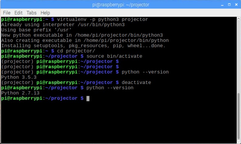
We can now create a new virtual environment for our project using the following command:
language:python
> virtualenv -p python3 projector
You can see in the command that we are specifying that when we run the python command while inside our new space, we want to run Python 3, and not what ever the system default is set to. We have also named our project projector because why not?
In case you’re new to virtualenv, once we’ve created our new environment we need to effectively “step inside,” or enter our new space. If you look at the directory structure created by the virtualenv command, you’ll notice a bin/ directory. This is where our Python executable lives, along with the file that tells our system to use this version of Python instead of our global system version. So in order to make this transition, we need to execute the following command
language:python
> source projector/bin/activate
Or, if you’d like to skip typing projector all the time:
language:python
> cd projector
> source bin/activate
You should see your prompt change once you’ve entered the environment.
language:python
(projector) pi@raspberry:~/projector $
The very next thing you should know is how to leave your development space. Once you’re finished and want to return to your normal, global python space, enter the following command:
language:python
> deactivate
That’s it! You’ve now created your protected development space that won’t change other things on your system, and won’t be changed by installing new packages, or running updates!
A note of clarification. This virtual environment is only for Python packages installed via pip, not apt-get. Packages installed with apt-get, even with the virtual environment activated, will be installed globally.
Continuing with our project, we will need to activate our development environment again.
language:python
> source bin/activate
We will need to add some dependencies. While putting together this tutorial, I found that there were some global dependencies that we need:
language:python
> sudo apt-get install libcblas.so.3
> sudo apt-get install libatlas3-base
> sudo apt-get install libjasper-dev
Now to install OpenCV for our project, along with a library for the Pi Camera, and some image utilities.
language:python
> pip install opencv-contrib-python
> pip install "picamera[array]"
> pip install imutils
We’re installing pre-built binaries for OpenCV here. These libraries are unofficial, but it’s not something to worry about, it just means they are not endorsed or supported directly by the folks at OpenCV.org. The alternative is to compile OpenCV from source, which is a topic for another tutorial.
We can install dlib in the same way. This also has a pre-built binary available for the Raspberry Pi, which again saves us hours of time.
language:python
> pip install dlib
Camera calibration is one of those really important steps that shouldn't be overlooked. With the reduction in price of small cameras over the years, we've also seen a significant increase in the amount of distortion their optics introduce. Calibration allows us to gather the camera's intrinsic properties and distortion coefficients so we can correct it. The great thing here is that, as long as our optics or focus don't change, we only have to calibrate the camera once!
Another important general note about camera calibration that doesn't apply to our project, but can be very helpful is that camera calibration also allows us to determine the relationship between the camera's pixels and real world units (like millimeters or inches).
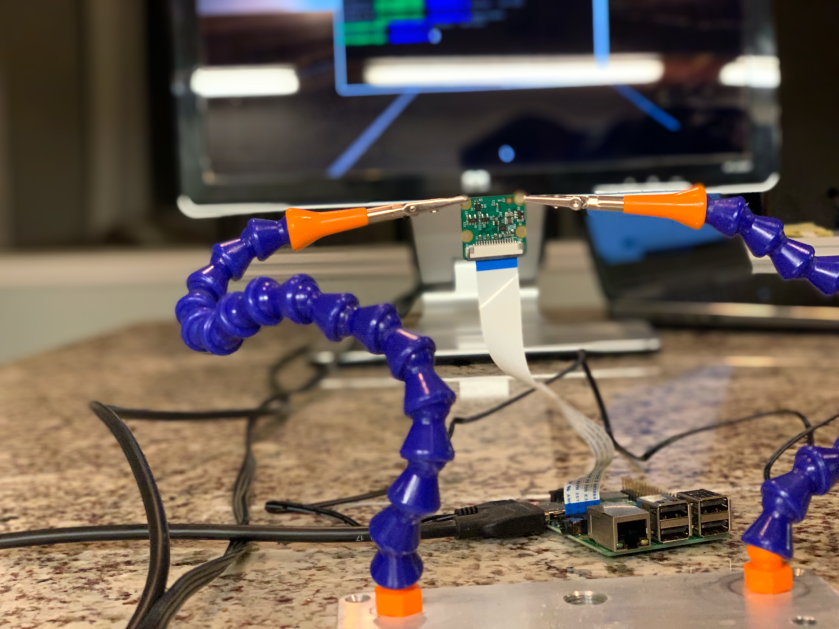
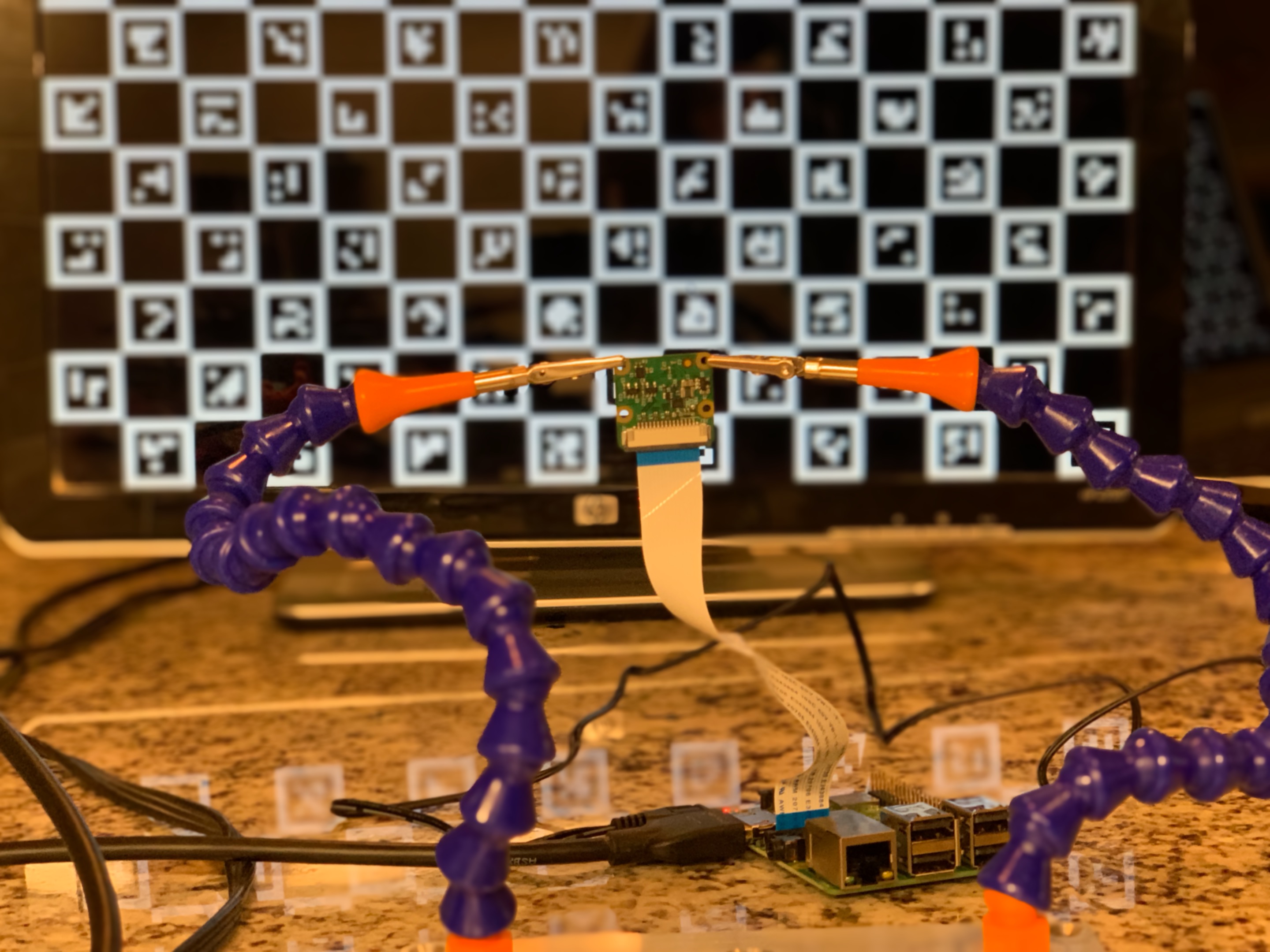
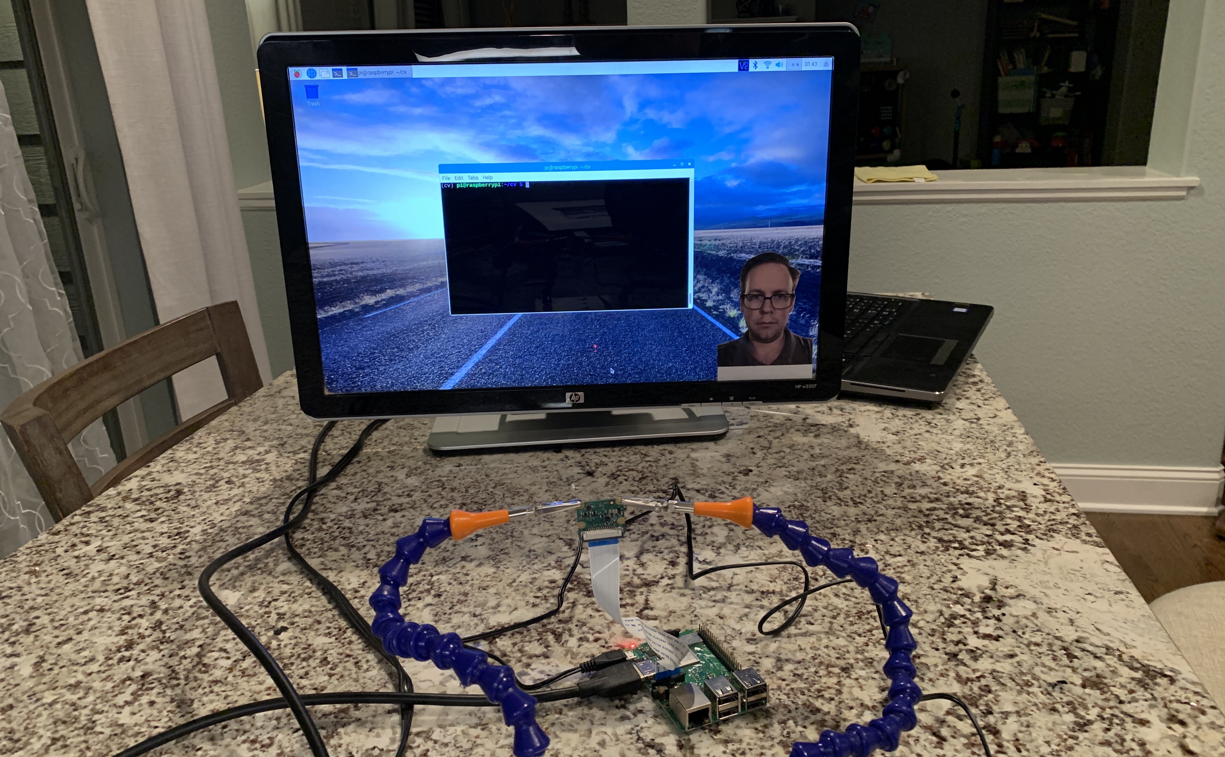
For my calibration setup, I mounted my Pi Camera module in some helping hands, and pointed it directly at my monitor. We need the calibration pattern to be on a flat surface, and instead of printing and mounting it, I figured this was easier. All of the documentation I found stressed the importance of capturing multiple view points of the calibration patter, but I'll admit, I only used one view point for this demo and you'll see that in the code. I've tried other calibration techniques gathering multiple views as well, and I found putting the calibration image on a tablet was useful. The screen of the tablet is very flat, and the fact that image is emitted light, not reflected, makes the ambient lighting not matter.
Let's start looking at the code
language:python
#! /usr/bin/env python3

"""
    A script to calibrate the PiCam module using a Charuco board
"""

import time
import json

import cv2

from cv2 import aruco
from imutils.video import VideoStream

from charuco import charucoBoard
from charuco import charucoDictionary
from charuco import detectorParams
We'll start all of our files with a #! statement to denote what program to use to run our scripts. This is only important if you change the file to be executable. In this tutorial we will be explicitly telling Python to run the file, so this first line isn't particularly important.
Moving on from there, we need to specify all of the import statements we will need for the code. You'll see I've used two different styles of import here: the direct import and the from. If you haven't run across this syntax before, it allows us to be specific about what we are including, as well as minimizes the typing required to access our imported code. A prime example is how we import VideoStream; we could have imported imutils directly and still accessed VideoStream like so:
language:python
import imuitls
vs = imutils.video.VideoStream
Another note about organization. I like to group my import statements by: included in Python, installed dependency, from statements included with Python (there are none in this case), from installed dependencies, and from created libraries. The charuco library is one I made to hold some values for me.
Now let's look at the functions we've put together to help us here.
language:python
def show_calibration_frame(frame):
    """
    Given a calibration frame, display the image in full screen
    Use case is a projector.  The camera module can find the projection region
    using the test pattern
    """
    cv2.namedWindow("Calibration", cv2.WND_PROP_FULLSCREEN)
    cv2.setWindowProperty("Calibration", cv2.WND_PROP_FULLSCREEN, cv2.WINDOW_FULLSCREEN)
    cv2.imshow("Calibration", frame)
This function allows us to easily use cv2 to show an image in full screen. There are several times while running this code where we will need to have a test pattern or image fill the available area. By naming our window we can find it later to destroy it.
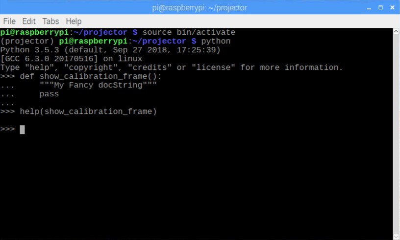
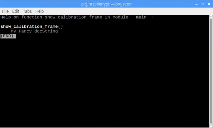
In Python, it's a good idea to add a docstring after the function declaration. This is just a string hanging out, but it's given some extra consideration. For example, if you document your code this way, the Python console can tell you information about a function by using the help command.
language:python
def hide_calibration_frame(window="Calibration"):
    """
    Kill a named window, the default is the window named "Calibration"
    """
    cv2.destroyWindow(window)
Here's our function that destroys our full screen image once we're done with it. The important thing to notice is that the names must match when the full screen image is created and destroyed. This is handled here by our default parameter, window="Calibration".
language:python
def save_json(data):
    """
    Save our data object as json to the camera_config file
    :param data: data to  write to file
    """
    filename = 'camera_config.json'
    print('Saving to file: ' + filename)
    json_data = json.dumps(data)
    with open(filename, 'w') as f:
        f.write(json_data)
Here we have a helper function that takes an object that we pass in, and writes it into a JSON file for us. If you're new to Python, it's worth mentioning the context manger we use when writing to the file.
The with open line above limits how long we have the file open in our script. We don't have to worry about closing the file after we're finished, as soon as we leave the scope of the with statement, the file is closed on our behalf.
language:python
def calibrate_camera():
    """
    Calibrate our Camera
    """
    required_count = 50
    resolution = (960, 720)
    stream = VideoStream(usePiCamera=True, resolution=resolution).start()
    time.sleep(2)  # Warm up the camera
Here we do some setup. We'll be looking to make sure we have at least 50 marker points for our calibration. We also set the camera resolution, as well as start the camera thread. We insert the sleep to make sure the camera stream is warmed up and providing us data before we move on.
language:python
   all_corners = []
    all_ids = []

    frame_idx = 0
    frame_spacing = 5
    success = False

    calibration_board = charucoBoard.draw((1680, 1050))
    show_calibration_frame(calibration_board)
Here is the last part of our setup. We make some lists to hold our discovered points, and set our frame offset. We don't really need to check every frame here, so it can help speed up our frame rate to only check every fifth frame.
We also load in our charuco board. Charuco boards are a combination of aruco markers (think along the lines of QR code marker) and a chessboard pattern. With the combination of both technologies, it is actually possible to get sub pixel accuracy.
You can find more information about the markers here.
language:python
    while True:
        frame = stream.read()
        gray = cv2.cvtColor(frame, cv2.COLOR_BGR2GRAY)

        marker_corners, marker_ids, _ = aruco.detectMarkers(
            gray,
            charucoDictionary,
            parameters=detectorParams)
Here we start the main loop where we will do our work. We start by getting a frame from the Pi Camera module and converting it to grayscale. Once we have our grayscale image, we feed it into OpenCV's detector along with the original dictionary we used when creating the board. Each marker is encoded with an ID that allows us to identify it, and when combined with the board placement, it gives us accurate information even if the board is partially occluded.
Another thing to point out here if you're new to Python is the unpacking syntax used for assignment. The aruco.detectMarkers function returns a tuple containing three values. If we provide three separate comma separated variables, Python will assign them in order. Here we are only interested in two of the values, so I've stuck an underscore in place as the last variable. An alternative would have been
language:python
return_val = aruco.detectMarkers(
    gray,
    charucoDictionary,
    parameters-detectorParams)
marker_corners = return_val[0]
marker_ids = return_val[1]
Let's continue with our original code.
language:python
       if len(marker_corners) > 0 and frame_idx % frame_spacing == 0:
            ret, charuco_corners, charuco_ids = aruco.interpolateCornersCharuco(
                marker_corners,
                marker_ids,
                gray,
                charucoBoard
                )
            if charuco_corners is not None and charuco_ids is not None and len(charuco_corners) > 3:
                all_corners.append(charuco_corners)
                all_ids.append(charuco_ids)

            aruco.drawDetectedMarkers(gray, marker_corners, marker_ids)
Next we check to see if we found any marker corners, and whether we've reached our fifth frame. If all is good, we do some processing on our detected corners, and make sure the results pass some data validation. Once everything checks out, we add the markers into the lists we set up outside of our loop.
Lastly, we draw our detected marker on our camera image.
language:python
        if cv2.waitKey(1) & 255 == ord('q'):
            break
Here we've added a check to see if the q key is pressed. If it is, we bail on the while loop. OpenCV is a little strange on how it wants to check keys, so we need to bitwise & the key value with 255 before we can compare it to the ordinal value of our key in question.
language:python
       frame_idx += 1
        print("Found: " + str(len(all_ids)) + " / " + str(required_count))

        if len(all_ids) >= required_count:
            success = True
            break
    hide_calibration_frame()
At this point we have ether successfully found the points we need, or we've hit the q key. In both cases, we need to stop showing our full screen calibration image.
language:python
    if success:
        print('Finished collecting data, computing...')

        try:
            err, camera_matrix, dist_coeffs, rvecs, tvecs = aruco.calibrateCameraCharuco(
                all_corners,
                all_ids,
                charucoBoard,
                resolution,
                None,
                None)
            print('Calibrated with error: ', err)

            save_json({
                'camera_matrix': camera_matrix.tolist(),
                'dist_coeffs': dist_coeffs.tolist(),
                'err': err
            })

            print('...DONE')
        except Exception as e:
            print(e)
            success = False
From here, if we've collected the appropriate number of points, we need to try to calibrate the camera. This process can fail, so I've wrapped it in a try/except block to ensure we fail gracefully if that's the case. Again, we let OpenCV do the heavy lifting here. We feed our found data into their calibrator, and save the output. Once we have our camera properties, we make sure we can get the later, by saving them off as a JSON file.
language:python
        # Generate the corrections
        new_camera_matrix, valid_pix_roi = cv2.getOptimalNewCameraMatrix(
            camera_matrix,
            dist_coeffs,
            resolution,
            0)
        mapx, mapy = cv2.initUndistortRectifyMap(
            camera_matrix,
            dist_coeffs,
            None,
            new_camera_matrix,
            resolution,
            5)
        while True:
            frame = stream.read()
            if mapx is not None and mapy is not None:
                frame = cv2.remap(frame, mapx, mapy, cv2.INTER_LINEAR)

            cv2.imshow('frame', frame)
            if cv2.waitKey(1) & 255 == ord('q'):
                break

    stream.stop()
    cv2.destroyAllWindows()
In this last section we leverage OpenCV to give us the new correction information we need from our camera calibration. This isn't exactly necessary for calibrating the camera, but as you see in the nested while loop, we are visualizing our corrected camera frame back on the screen. Once we've seen our image, we can exit by pressing the q key.
language:python
if __name__ == "__main__":
    calibrate_camera()
Here's our main entry point. Again, if you're new to Python, this if __name__ == "__main__": statement might look a bit weird. When you run a Python file, Python will run EVERYTHING inside the file. Another way to think about this is if you want a file loaded, but no logic executed, all code has to live inside of a class, function, conditional, etc. This goes for imported files as well. What this statement does is make sure that this code only runs if it belongs to the file that was called from the command line. As you'll see later, we have code in this same block in some of our files, and it allows us to import from them without running as if we were on the command line. It lets us use the same file as a command line program and a library at the same time.
Now let's take a look at what's in our imported charuco file.
language:python
#! /usr/bin/env python3

from cv2 import aruco

inToM = 0.0254

# Camera calibration info
maxWidthIn = 17
maxHeightIn = 23
maxWidthM = maxWidthIn * inToM
maxHeightM = maxHeightIn * inToM

charucoNSqVert = 10
charucoSqSizeM = float(maxHeightM) / float(charucoNSqVert)
charucoMarkerSizeM = charucoSqSizeM * 0.7
# charucoNSqHoriz = int(maxWidthM / charucoSqSizeM)
charucoNSqHoriz = 16

charucoDictionary = aruco.getPredefinedDictionary(aruco.DICT_4X4_100)
charucoBoard = aruco.CharucoBoard_create(
    charucoNSqHoriz,
    charucoNSqVert,
    charucoSqSizeM,
    charucoMarkerSizeM,
    charucoDictionary)

detectorParams = aruco.DetectorParameters_create()
detectorParams.cornerRefinementMaxIterations = 500
detectorParams.cornerRefinementMinAccuracy = 0.001
detectorParams.adaptiveThreshWinSizeMin = 10
detectorParams.adaptiveThreshWinSizeMax = 10
I've put up the relevant portions of the file here. There's a bit more that is used in another file where I was attempting an alternative approach, so you can just disregard that for now. As you can see, the file is mostly just constants and a little work to build our board and set up our parameters. One thing to notice here is our code does not live inside a class, function, or conditional. This code is run at import time, and before any of our main code is run! This way we can make sure all of our values are correct and available to us when we're ready to use them.
The full working examples can be found in the GitHub repo as the aruco_calibration.py and charuco.py files.
Now that we have our camera calibration information, the next step in our projector project is determining where our projected image is within the camera view. There are a couple ways to do this. I started off going down the road of projecting another charuco board like we used in the calibration step, but I didn't like the approach because of the extra math to extrapolate the image corners from the marker corners. Instead we'll project a white image, finding the edges and contours in what our camera sees, and pick the largest one with four corners as our projected image. The biggest pitfall here is lighting, so during this step, it might help to dim the lights if you're having trouble.
language:python
#! /usr/bin/env python3
"""
    This program calculates the perspective transform of the projectable area.
    The user should be able to provide appropriate camera calibration information.
"""

import argparse
import json
import time

import cv2
import imutils
import numpy as np

from imutils.video import VideoStream
This beginning part will hopefully start to look familiar:
language:python
def show_full_frame(frame):
    """
    Given a frame, display the image in full screen
    :param frame: image to display full screen
    """
    cv2.namedWindow('Full Screen', cv2.WND_PROP_FULLSCREEN)
    cv2.setWindowProperty('Full Screen', cv2.WND_PROP_FULLSCREEN, cv2.WINDOW_FULLSCREEN)
    cv2.imshow('Full Screen', frame)


language:python
def hide_full_frame(window='Full Screen'):
    """
    Kill a named window, the default is the window named 'Full Screen'
    :param window: Window name if different than default
    """
    cv2.destroyWindow(window)
You'll notice that, while the window name is changed, these are identical to the previous file. Normally I would make a shared module where I would put these helper functions that are re-used, but for the sake of this tutorial, I've left most things in the same file.
language:python
def get_reference_image(img_resolution=(1680, 1050)):
    """
    Build the image we will be searching for.  In this case, we just want a
    large white box (full screen)
    :param img_resolution: this is our screen/projector resolution
    """
    width, height = img_resolution
    img = np.ones((height, width, 1), np.uint8) * 255
    return img
When we go searching for our camera image for our project-able region, we will need some way to define that region. We'll do that by using our projector or monitor to display a bright white image that will be easy to find. Here we have a function that builds that white screen for us. We pass in the projector or screen resolution, and use NumPy to create an array of pixels, all with the value 255. Once we've created the image, we pass it back to the calling function.
language:python
def load_camera_props(props_file=None):
    """
    Load the camera properties from file.  To build this file you need
    to run the aruco_calibration.py file
    :param props_file: Camera property file name
    """
    if props_file is None:
        props_file = 'camera_config.json'
    with open(props_file, 'r') as f:
        data = json.load(f)
    camera_matrix = np.array(data.get('camera_matrix'))
    dist_coeffs = np.array(data.get('dist_coeffs'))
    return camera_matrix, dist_coeffs
You'll remember that in our last section, we calibrated our camera and saved the important information in a JSON file. This function lets us load that file and get the important information from it.
language:python
def undistort_image(image, camera_matrix=None, dist_coeffs=None, prop_file=None):
    """
    Given an image from the camera module, load the camera properties and correct
    for camera distortion
    """
    resolution = image.shape
    if len(resolution) == 3:
        resolution = resolution[:2]
    if camera_matrix is None and dist_coeffs is None:
        camera_matrix, dist_coeffs = load_camera_props(prop_file)
    resolution = resolution[::-1]  # Shape gives us (height, width) so reverse it
    new_camera_matrix, valid_pix_roi = cv2.getOptimalNewCameraMatrix(
        camera_matrix,
        dist_coeffs,
        resolution,
        0
    )
    mapx, mapy = cv2.initUndistortRectifyMap(
        camera_matrix,
        dist_coeffs,
        None,
        new_camera_matrix,
        resolution,
        5
    )
    image = cv2.remap(image, mapx, mapy, cv2.INTER_LINEAR)
    return image
In this function, we are wrapping up our image correction code from our preview during calibration into a more portable form. We start by pulling information about our frame to determine the height and width of the image in pixels. Next we check if we have our camera calibration information. Don't be confused by the function signature, where we can pass in our parameters, or the the file name. This function is used in more than one place, and I decided to make it so you could call the function with the information you had at the time.
Once we have the information we need, we have to reverse the height and width of our resolution. The shape property returns the information in a (height, width, ...) format.
Next we calculate the correction parameters for our image. I'll just point out that this is demo code, and far from ideal. You might notice that every time this function is called, we process the calibration information. That's a lot of extra processing that we end up doing in every camera frame that we want to use. Moving the correction parameters out so they are only calculated once would be a major improvement that would probably improve the overall frame rate of the final project.
Lastly, we correct the image, and return it to the calling function.
language:python
def find_edges(frame):
    """
    Given a frame, find the edges
    :param frame: Camera Image
    :return: Found edges in image
    """
    gray = cv2.cvtColor(frame, cv2.COLOR_BGR2GRAY)
    gray = cv2.bilateralFilter(gray, 11, 17, 17)  # Add some blur
    edged = cv2.Canny(gray, 30, 200)  # Find our edges
    return edged
This function helps us find the edges in our camera image. We start by reducing the number of channels we need to process by converting the image to grayscale. After that, we add some blur into the image to help us get more consistent results. Finally, we compute the edges and return our results.
One thing that I've noticed as I worked through this demo is the amount of "Magic Numbers" that are included in code. "Magic Numbers" are the constants that appear in the code without explanation. For example, in the code above we call the cv2.Canny function with the image frame, but also with the numbers 30 and 200. What are they? Why are they there? Why doesn't the code work without them? These are all questions to avoid in a tutorial, and while I've tried to keep them to a minimum, the libraries we use, like OpenCV, that come from C++, aren't always graceful about their requirements. When it comes to the library functions and methods, I'd recommend browsing the documentation pages like this one, and know that in many cases (like the one above) I've borrowed directly from example code, without fully understanding the importance either.
language:python
def get_region_corners(frame):
    """
    Find the four corners of our projected region and return them in
    the proper order
    :param frame: Camera Image
    :return: Projection region rectangle
    """
    edged = find_edges(frame)
    # findContours is destructive, so send in a copy
    image, contours, hierarchy = cv2.findContours(edged.copy(), cv2.RETR_TREE, cv2.CHAIN_APPROX_SIMPLE)
    # Sort our contours by area, and keep the 10 largest
    contours = sorted(contours, key=cv2.contourArea, reverse=True)[:10]
    screen_contours = None

    for c in contours:
        # Approximate the contour
        peri = cv2.arcLength(c, True)
        approx = cv2.approxPolyDP(c, 0.02 * peri, True)

        # If our contour has four points, we probably found the screen
        if len(approx) == 4:
            screen_contours = approx
            break
    else:
        print('Did not find contour')
    # Uncomment these lines to see the contours on the image
    # cv2.drawContours(frame, [screen_contours], -1, (0, 255, 0), 3)
    # cv2.imshow('Screen', frame)
    # cv2.waitKey(0)
    pts = screen_contours.reshape(4, 2)
    rect = order_corners(pts)
    return rect
This function takes our camera frame, finds the contours within the image, and returns our projection region. We start by calling out to our function that finds the edges within our image. Once we've found our edges, we move on to identifying our contours (or outlines). Here again, you'll find the the OpenCV library has made things easy for us.
Now we need to identify our projection region. I tried many different ways to find our region including feature detection between a reference image and our projected region, and projecting a charuco board to identify the markers, but settled on using contours because they were much simpler and much more reliable. At this point in the code, we have our identified contours, but we need to sort them into some sort of order. We use the Python sorted() function to allow us to do a custom sort in the following way: sorted(what_to_sort, key=how_to_sort, reverse=biggest_first)[:result_limit]. I've added a limit to the number of results we carry around because we only care about the biggest regions in the image (our projection region should be one of the biggest things we can see with four corners).
Once we have our sorted contours, we need to iterate through them, clean up the contour, and find our four-corner winner. We check the number of corners with the len(approx) == 4: command above, and if we've found our box, we save the data and stop searching with our break command.
Our last step is to reshape our data into a nicer matrix and put the corner points into the correct order for processing later, before returning it to the calling function.
If all goes well, and you uncomment the lines in the file, you should have something like this:
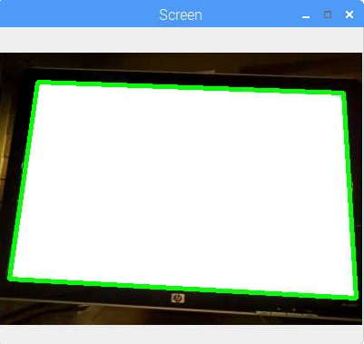
language:python
def order_corners(pts):
    """
    Given the four points found for our contour, order them into
    Top Left, Top Right, Bottom Right, Bottom Left
    This order is important for perspective transforms
    :param pts: Contour points to be ordered correctly
    """
    rect = np.zeros((4, 2), dtype='float32')

    s = pts.sum(axis=1)
    rect[0] = pts[np.argmin(s)]
    rect[2] = pts[np.argmax(s)]

    diff = np.diff(pts, axis=1)
    rect[1] = pts[np.argmin(diff)]
    rect[3] = pts[np.argmax(diff)]
    return rect
This function uses the sum and diff along with the min and max to figure out which corner goes where, matching the order that we'll need to use later to transform our space.
language:python
def get_destination_array(rect):
    """
    Given a rectangle return the destination array
    :param rect: array of points  in [top left, top right, bottom right, bottom left] format
    """
    (tl, tr, br, bl) = rect  # Unpack the values
    # Compute the new image width
    width_a = np.sqrt(((br[0] - bl[0]) ** 2) + ((br[1] - bl[1]) ** 2))
    width_b = np.sqrt(((tr[0] - tl[0]) ** 2) + ((tr[1] - tl[1]) ** 2))

    # Compute the new image height
    height_a = np.sqrt(((tr[0] - br[0]) ** 2) + ((tr[1] - br[1]) ** 2))
    height_b = np.sqrt(((tl[0] - bl[0]) ** 2) + ((tl[1] - bl[1]) ** 2))

    # Our new image width and height will be the largest of each
    max_width = max(int(width_a), int(width_b))
    max_height = max(int(height_a), int(height_b))

    # Create our destination array to map to top-down view
    dst = np.array([
        [0, 0],  # Origin of the image, Top left
        [max_width - 1, 0],  # Top right point
        [max_width - 1, max_height - 1],  # Bottom right point
        [0, max_height - 1],  # Bottom left point
        ], dtype='float32'))
    return dst, max_width, max_height
This function builds the matrix we will need to transform from our skewed view of the projection region into a perspective-corrected, top-down view that we need to accurately manipulate our data.
We start by computing the distance between our x coordinates on the top and bottom of the image. Next, we do the same with our y coordinates on the left and right side of the image. Once these calculations are finished, we save the max width and height to use in our matrix creation.
To create our matrix, we provide the computed values of our four corners based on our max width and height.
Finally we return the important data back to the calling function.
language:python
def get_perspective_transform(stream, screen_resolution, prop_file):
    """
    Determine the perspective transform for the current physical layout
    return the perspective transform, max_width, and max_height for the
    projected region
    :param stream: Video stream from our camera
    :param screen_resolution: Resolution of projector or screen
    :param prop_file: camera property file
    """
    reference_image = get_reference_image(screen_resolution)

    # Display the reference image
    show_full_frame(reference_image)
    # Delay execution a quarter of a second to make sure the image is displayed
    # Don't use time.sleep() here, we want the IO loop to run.  Sleep doesn't do that
    cv2.waitKey(250)

    # Grab a photo of the frame
    frame = stream.read()
    # We're going to work with a smaller image, so we need to save the scale
    ratio = frame.shape[0] / 300.0

    # Undistort the camera image
    frame = undistort_image(frame, prop_file=prop_file)
    orig = frame.copy()
    # Resize our image smaller, this will make things a lot faster
    frame = imutils.resize(frame, height=300)

    rect = get_region_corners(frame)
    rect *= ratio  # We shrank the image, so now we have to scale our points up

    dst, max_width, max_height = get_destination_array(rect)

    # Remove the reference image from the display
    hide_full_frame()

    m = cv2.getPerspectiveTransform(rect, dst)

    # Uncomment the lines below to see the transformed image
    # wrap = cv2.warpPerspective(orig, m, (max_width, max_height))

    # cv2.imshow('all better', wrap)
    # cv2.waitKey(0)
    return m, max_width, max_height
Here's where we start to put the pieces together. Take a look at the in-line comments here, as they'll probably be more helpful than a summary paragraph at the end.
We start by building our solid white image to the resolution of our screen or projector. Once we have that, we display it for our camera to see. We delay our image capture a quarter-second to make sure the image has time to get up on the display, then snap a frame.
Working with full size images is slow, so we compute and save a resize ratio, then make our frame smaller. Once we've computed the corners of our projection region, we use our saved ratio to make our found region match the locations in our original image.
Using our new corner data, we call our function that computes the destination array for our perspective transform. We stop displaying our reference (white) image, and then use the returned data to calculate our perspective transform.
You'll see some lines here that are commented out. If you'd like to see the corrected image, uncomment these lines. This can be helpful to visualize what is happening at each step.
Finally we return our perspective transform and the max width and height.
language:python
def parse_args():
    """
    A command line argument parser
    :return:
    """
    ap = argparse.ArgumentParser()
    # Camera frame resolution
    ap.add_argument('-cw', '--camera_width', type=int, default=960,
                    help='Camera image width')
    ap.add_argument('-ch', '--camera_height', type=int, default=720,
                    help='Camera image height')
    # camera property file
    ap.add_argument('-f', '--camera_props', default='camera_config.json',
                    help='Camera property file')
    # Screen resolution
    ap.add_argument('-sw', '--screen_width', type=int, default=1680,
                    help='Projector or screen width')
    ap.add_argument('-sh', '--screen_height', type=int, default=1050,
                    help='Projector or screen height')
    return vars(ap.parse_args())
This next function is just a way to use Python's argparse to build a command line parser. This allows us to feed in these commands and override settings without the need for changing the code. You might notice that I have flags for camera width and camera height. Parsing values with spaces and such is tricky, so instead of passing in a tuple (think (width, height)) I just set each individually.
language:python
>fbset -s
If you're unsure what your screen resolution is, this bash command makes it easy to find.
language:python
if __name__ == '__main__':
    args = parse_args()
    # Camera frame resolution
    resolution = (args.get('camera_width'), args.get('camera_height'))

    stream = VideoStream(usePiCamera=True, resolution=resolution).start()

    time.sleep(2)  # Let the camera warm up

    screen_res = (args.get('screen_width'), args.get('screen_height'))
    get_perspective_transform(stream, screen_res, args.get('camera_props'))
    stream.stop()
    cv2.destroyAllWindows()
Here is the main control of our program. You can see the main program flow here. We start by gathering our arguments and starting our video stream. After that, we call our function get_perspective_transform and pass it the information it needs. Once we have our information, we clean up by stopping our camera stream and cleaning up any windows that might be open.
Now that we have found the contours of our project-able region, we can work on de-skewing the image, or calculating and applying the perspective transform we need to take this trapezoidal region and making it square. This artifacting is introduced by the fact that we cannot have the camera and projector directly on axis with each other. We need to do this correction so that we can accurately place the image sprites in the real world.
The code to do this now that we have all our information is fairly straightforward.
frame = warpPerspective(frame, m, (maxWidth, maxHeight))
This accomplishes our de-skew, and crops our image to the region in question. Another way to think of what this does is that it gives us back only the part of our image that is our project-able region. Everything else is discarded. This is important because we will need to look for faces within this region, and now that the region is square (not trapezoidal) we can start to calculate where our sprites need to go.
Ok, now that we've identified our project-able region, it's time to watch for and identify faces! We don't care about the regions of the image that the camera can see but can't interact with, so we only need to work with the corrected and cropped portion that is our project-able region, which we found in the last section.
Detecting faces is where dlib really excels. In the past I've used openCV for face detection (Harr cascades) and while it gets the job done, the detected faces from dlib are far more flexible, and give information about facial features, among other things.
Setting up our face detector is as follows:
language:python
detector = dlib.get_frontal_face_detector()
predictor = dlib.shape_predictor(args.get('predictor'))
You can use a variety of face predictors, but I've used the generic predictor available directly from dlib here.
Don't forget to extract your download:
language:python
> bzip2 -d shape_predictor_68_face_landmarks.dat.bz2
Here's an example of getting our faces from our image:
language:python
rects = detector(image, 0)
for mark in rects:
    shape = predictor(image, mark)
    shape = face_utils.shape_to_np(shape)
This is the basic usage for finding faces. You'll see when we put this all together how we can use this data to overlay our sprites.
Now that we've found what we're looking for (in this case faces), it's time to build the image we want to project back into the world. If you think about it, we don't want to project the image captured from the camera back out into the world. If you were standing in front of the camera and projector, you wouldn't want the image of your own face projected back on top of it in addition to the sprite we will add. To overcome this, we will create a black image that matches our projector resolution that we will add our sprite into. This is where using a monitor instead of a projector changes our setup a little.
If you'd like to continue using a monitor, I'd suggest cutting out a small printout of a head and taping it to something like a Popsicle stick. As you move the head around in front of the monitor, our project should move the sprite around behind it.
One of the last pieces we need to tackle is mapping from the pixel positions in our captured image to the pixel positions in our image that we will project.
Where we need pixel values, I used the numpy function interp():
language:python
    for index, (x, y) in enumerate(shape):
        # We need to map our points to the new image from the original
        new_x = int(np.interp(x, [0, f_width], [0, d_width]))
        new_y = int(np.interp(y, [0, f_height], [0, d_height]))
where shape is a list of our facial feature points in (x, y) format, f_width and f_height are the captured image width and height, and d_width and d_height are our display width and height.
Other places I just multiplied by the a scale ratio:
language:python
face_width = int(mark.width() * (d_width/f_width))
where mark is a detected face object provided by dlib, and d_width and f_width are the same as above.
We want to avoid fractional pixels, so it's good to cast our interpolated points to an int() so they have no decimal points.
Now that we've figured out how to map between our two spaces, we can finally create our new image! We will start from a blank black image, and merge our sprite image on top. We want to avoid projecting what the camera sees back on top of the real world thing it saw, so effectively a black image is no projection.
Interesting note here, if you are in an environment that has poor lighting and you run into issues with the camera seeing and detecting faces, you can change the black background to varying shades of gray to have the projector create its own lighting. You add utility at the expense of making the project-able region more pronounced.
Let's run through the complete code for our project.
language:python
#! /bin/env python3

from imutils.video import VideoStream
from imutils import face_utils
from imutils import rotate_bound
from contour_perspective_calibrator import load_camera_props
from contour_perspective_calibrator import undistort_image
from contour_perspective_calibrator import get_perspective_transform
from contour_perspective_calibrator import show_full_frame

import argparse
import math
import time
import dlib
import cv2
import numpy as np
In addition to our normal imports, you'll notice that I'm reaching back into our calibration file to reuse the load_camera_props, undistory_image, get_perspective_transfom, and show_full_frame functions. No need to copy and paste.
language:python
def build_image(frame, display_resolution, markers, predictor, sprite_path):
    """
    Function to build our marker image
    We're building a black image and adding the proper markers to it, so that
    when it's projected, only the markers display on the target
    :param frame: corrected and transformed image (already b&w)
    :param display_resolution: the current displayed or projected screen resolution
    :param markers: Found detector markers
    :param predictor: the loaded facial predictor
    :param sprite_path: the location of the sprite
    :return: built image
    """
    d_width, d_height = display_resolution
    f_height, f_width = frame.shape
    img = np.zeros((d_height, d_width, 3), np.uint8)
    for mark in markers:
        shape = predictor(frame, mark)
        shape = face_utils.shape_to_np(shape)
        # Grab some info from the detected face.
        # The top and left give us the origin
        # The width and height give us scale/size
        # DON'T FORGET we need to map the values back to screen resolution
        face_left = int(np.interp(mark.left(), [0, f_width], [0, d_width]))
        face_top = int(np.interp(mark.top(), [0, f_height], [0, d_height]))
        face_width = int(mark.width() * (d_width/f_width))
        face_height = int(mark.height() * (d_height/f_height))

        scaled_shape = np.copy(shape)
        for index, (x, y) in enumerate(shape):
            # We need to map our points to the new image from the original
            new_x = int(np.interp(x, [0, f_width], [0, d_width]))
            new_y = int(np.interp(y, [0, f_height], [0, d_height]))
            scaled_shape[index] = [new_x, new_y]
            # Uncomment the line below to set the point projected on the target
            # cv2.circle(img, (new_x, new_y), 1, (255, 255, 255), -1)
        inclination = calc_incl(scaled_shape[17], scaled_shape[26])  # get the info from eyebrows
        apply_sprite(img, face_width, face_left, face_top, inclination, sprite_path)
    return img
Here is where we build the full image we will project back onto our detected face. We start by unpacking the display and frame resolutions into their widths and heights.
Next we create our blank image. We use the np.zeros function to create an array with three channels (RGB) and all values set to zero for black.
Our next step is to step through all of our detected faces. In our loop, we use the dlib predictor to find our key facial points and convert them to a numpy array.
We need to gather some information about our found faces, so we pull the parameters from our face object, mark in the code above. We also perform our space mapping here, so that our locations and values are already in our display resolution.
In the next few lines, we make a copy of our facial features array, and transform each of the points to our display space. If you'd like to see where each of the points lands, uncommenting the cv2.circle command will draw little circles on each of the points. This can be useful to visualize where each of the points is in relation to our detected face. I used this to verify that we were accurately displaying our image on top of a real face.
In the last few steps, we calculate face tilt by looking at our detected face's eyebrows. Once we've found the angle, we apply our sprite to our black image and hand it back to the calling function.
One interesting thing of note: we don't need to save the result of apply_sprite(). Everything in Python is pass-by reference, so when we make modifications to img inside the function, we are modifying the same object img that exists in this scope.
language:python
def apply_sprite(image, width, x, y, angle, sprite_file):
    """
    Given an image, add our sprite
    :param image: our image to be projected
    :param width: Target face width
    :param x: Face location left
    :param y: Face location top
    :param angle: face tilt
    :param sprite_file: the filename of our sprite
    :return: projection image
    """
    sprite = cv2.imread(sprite_file, cv2.IMREAD_UNCHANGED)
    sprite = rotate_bound(sprite, angle)
    sprite, y_final = transform_sprite(sprite, width, y)
    sp_h, sp_w = sprite.shape[:2]
    img_h, img_w = image.shape[:2]

    if y_final + sp_h >= img_h:  # Off the page to the bottom
        sprite = sprite[0:img_h-y_final, :, :]
    if x + sp_w >= img_w:  # Off the page to the right
        sprite = sprite[:, 0:img_w-x, :]
    if x < 0:  # Off the page to the left
        sprite = sprite[:, abs(x)::, :]
        sp_w = sprite.shape[1]
        x = 0

    # loop through and combine the image and sprite based on the sprite alpha values
    for chan in range(3):
        image[y_final:y_final+sp_h, x:x+sp_w, chan] = \
                sprite[:, :, chan] * (sprite[:, :, 3] / 255.0) + \
                image[y_final:y_final+sp_h, x:x+sp_w, chan] * \
                (1.0 - sprite[:, :, 3] / 255.0)
    return image
Applying the sprite to our base image is fairly straightforward, with a few special pieces to consider. We start by reading our image from file. There is a lot of overhead with this, and if I were to do a second version of this code, I think I would make a class where I could store the loaded image and skip reloading it each frame. Once we have our sprite image, we rotate it in relation to head tilt, and the scale and move our sprite to the correct location.
Once we know where the sprite will be positioned in the final image, we need to crop it to the bounds of the image we will project back onto our face later. We do this with the series of if statements.
Lastly, we loop through our channels (RGB), and use the sprite's alpha values to overlay the images, pixel by pixel. Remember that the range(3) function will return a list from 0-2 inclusive, or [0, 1, 2] for three total values. When we use sprite channel 3, we're accessing the alpha value. This is why we need to load the image with cv2.IMREAD_UNCHANGED to preserve this data. As a note, when we use the backslash \, we are breaking a single line onto multiple lines. If you don't use this, Python will give you a syntax error.
language:python
def transform_sprite(sprite, width, y):
    """
    Match the size of our sprite to our detected face width
    :param sprite: the fun image
    :param width: the width we need to adjust to
    :param y: Vertical position of the sprite
    :return: the sprite (may be modified) and the new origin
    """
    manual_adjust = 1.2  # Added this to account for the extra width of the sprite
    sp_h, sp_w = sprite.shape[:2]
    ratio = (float(width) * manual_adjust)/float(sp_w)
    sprite = cv2.resize(sprite, (0, 0), fx=ratio, fy=ratio)
    sp_h, sp_w = sprite.shape[:2]
    y_origin = y - sp_h
    if y_origin < 0:  # the sprite is off the page, so cut it off
        sprite = sprite[abs(y_origin)::, :, :]
        y_origin = 0
    return sprite, y_origin
In this function, we scale our sprite to match the size of our detected face.
Our first parameter, manual_adjust, I added after the fact because we want our sprite to extend a little on both sides of the detected face. It looked a bit weird with the sprite exactly the same with as the face. There are situations where it would be desired to have this be the case, but I found that using a hat wasn't one of them.
After setting our manual scaling factor, we pull size information from our loaded sprite, and compute our scaling ratio.
We use OpenCV to scale our sprite, providing the ratios we calculated.
Next we look at y_origin, or the placement of our sprite. Remember that y=0 is located at the top of our screen, and positive y values go down our view area. We subtract the height of our scaled sprite from our y placement to see if it's negative (off the top of the page). If it is, we cut off the top of our sprite, and reset the calculated y_origin value to be 0 or the top of the image.
Finally we return the sprite and its calculated placement in the final image.
language:python
def calc_incl(point1, point2):
    """
    Calculate the angle of inclination between two points
    :param point1:
    :param point2:
    :return: the angle in question
    """
    x1, y1 = point1
    x2, y2 = point2
    incl = 180/math.pi*math.atan((float(y2-y1)/(x2-x1)))
    return incl
Here we just calculate the angle between two points. In our use case, this angle should be head tilt computed from the location of the eyebrows.
language:python
def parse_args():
    ap = argparse.ArgumentParser()
    ap.add_argument('-f', '--camera_props', default='camera_config.json',
                    help='Camera property file')
    ap.add_argument('-cw', '--camera_width', type=int, default=960,
                    help='Camera image width')
    ap.add_argument('-fh', '--camera_height', type=int, default=720,
                    help='Camera image height')
    ap.add_argument('-sw', '--screen_width', type=int, default=1824,
                    help='Projector or screen width')
    ap.add_argument('-sh', '--screen_height', type=int, default=984,
                    help='Projector or screen height')
    ap.add_argument('-s', '--sprite', default='santa_hat.png',
                    help='Our image sprite')
    ap.add_argument('-p', '--predictor',
                    default='shape_predictor_68_face_landmarks.dat',
                    help='Face landmark shape predictor')

    return vars(ap.parse_args())
Here we set up what options we can provide from the command line, and their defaults if no option is provided. This helps us be more flexible with our program, avoiding the need to make code changes for each use case. One thing to point out – I've set the default for my sprite file to be 'santa_hat.png'. You could use any image file here, but the thing that makes a good file is a transparent background.
language:python
if __name__ == '__main__':
    args = parse_args()
    print('Loading facial landmark predictor...')
    detector = dlib.get_frontal_face_detector()
    predictor = dlib.shape_predictor(args.get('predictor'))
    print('Camera sensor warming up...')
    camera_resolution = (args.get('camera_width'), args.get('camera_height'))
    vs = VideoStream(usePiCamera=True, resolution=camera_resolution).start()
    time.sleep(2)

    prop_file = args.get('camera_props')
    cameraMatrix, distCoeffs = load_camera_props(prop_file)
    screen_resolution = (args.get('screen_width'), args.get('screen_height'))
    m, maxWidth, maxHeight = get_perspective_transform(
        vs,
        screen_resolution,
        prop_file
    )

    while True:
        frame = vs.read()
        frame = undistort_image(frame, cameraMatrix, distCoeffs)  # Remove camera distortion
        frame = cv2.warpPerspective(frame, m, (maxWidth, maxHeight))
        gray = cv2.cvtColor(frame, cv2.COLOR_BGR2GRAY)

        rects = detector(gray, 0)

        image = build_image(gray, screen_resolution, rects, predictor, args.get('sprite'))

        show_full_frame(image)
        key = cv2.waitKey(1) & 0xFF

        if key == ord('q'):
            break

    cv2.destroyAllWindows()
    vs.stop()
We finally get to put the whole thing together! When we kick off this script from the command line, we start by pulling together all of the arguments provided and their defaults. We provide some messaging to the user giving some status indication, and load our facial detector and predictor from dlib.
Next, we grab the resolution for our camera from the arguments, and create our video stream. Since the stream is running in a separate thread, we sleep to make sure it has time to start before we try to get data from it.
We load our camera calibration properties from file, and gather our display resolution.
In the next line, we find our projection region and the transforms we need to correct the frames that we capture.
At this point, our setup has finished, and we can begin processing frames and building our projection image!
We step into a while True: loop to continue processing images until we press the q key.
In our loop, we get a frame from our video stream and remove its camera distortion. After that, we undistort our frame, and crop it down to our region of interest (only the area that we can project onto).
From this point, we get a grayscale copy of the image, and pass it to our face detector. We pass the returned faces into our image builder along with our cropped image, the display resolution, and our trained predictor (provided by dlib), and get back the image we need to project or display on our monitor.
Now that we have our image, we need to display it. We use our show_full_frame() function to do that for us. The next line, key = cv2.waitKey(1) & 0xFF allows OpenCV to update the projected image on the screen, as well as look for any pressed key. If a key has been pressed, and the key is q, then we break out of our while loop, clean up our windows and exit the program!
To run our finished project, all you need to do is type:
language:python
> python face_detector.py
My hope is that you see something close to what I have here. Oh, I didn't mention it before, but since we loop through our found faces, nothing says this is limited to one face at a time!
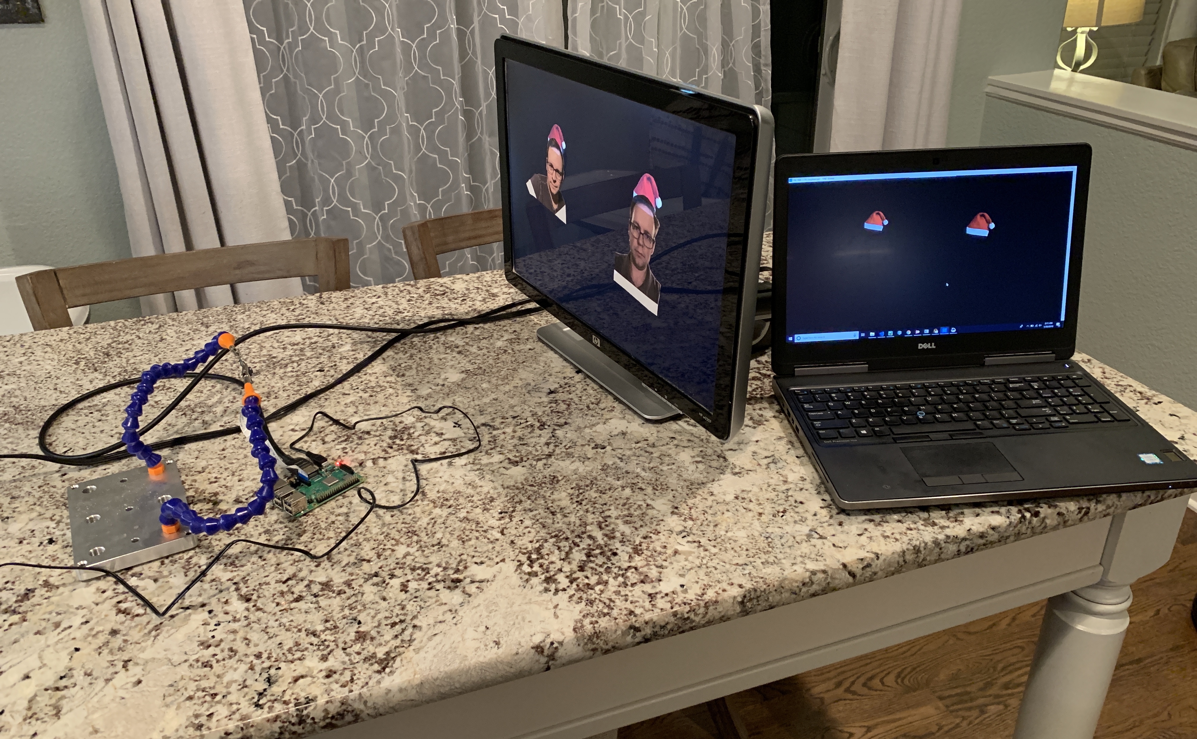
So what about the projector? Did that work too? Well, we defined success as when I could be in front of the projector and it could find me and put a hat on me... so yes! Once more with feeling:
My hope is that you found this tutorial informative and helpful in understanding some of what you can do with computer vision on a Raspberry Pi. If you have any questions or need any clarifications, please comment, and I'll try to clarify where I can.
Want to learn more about Python? Hvae a look at some of the resources below!
Looking for even more inspiration? Check out these other Raspberry Pi projects:
Or check out some of these blog posts for ideas:
learn.sparkfun.com | CC BY-SA 3.0 | SparkFun Electronics | Niwot, Colorado